The Story of OpenSprinkler: an Open-Source Web-Based Sprinkler Controller

Last week I wrote a short story on OpenSprinkler for the Make Magazine blog. It’s about how learning Arduino inspired me to invent the OpenSprinkler. Check out the blog post at the link below:

Thanks to everyone who helped and contributed to this project!

This year we will be having a booth at the Bay Area Maker Faire again. If you are going there too, make sure to drop by our booth and check out OpenSprinkler, SquareWear, AASaver, and the upcoming goodies. Thanks!

Reverse Engineer Wireless Temperature / Humidity / Rain Sensors — Part 3

Continuing from Part 1 and Part 2, this is the third and last post about how I reverse engineered a few off-the-shelf wireless temperature, humidity, and rain sensors, and used an Arduino to listen to and decode the sensor data. Update: RPi is also supported now! Check the provided programs at the end of this post.

Wireless Rain Sensor

Raw Waveform. There are several different wireless rain sensors on the market. My first target was an Acu-Rite 00875W rain gauge. I bought it two years ago and I don’t know if it’s still available now. This sensor turns out to be a huge pain. The main problem is that I can’t even register a consistent reading at 0 — every time I pop in the battery, I get a different signal that seems to have nothing to do with the previous readings. Also, the 0/1 bit patterns are completely unclear from the captured waveform — there are at least 4 or 5 different wavelengths. Here are two examples of the captured waveforms. They look nothing alike, even though both were captured right after the batteries are popped in and no rain has been detected.

IMG_0055rain_sensor_waveform0

After pulling my hair for a couple of days and finding no clue at all, I decided to give it up and try a different model. This time I bought an Acu-Rite 00899 wireless rain gauge. It’s probably worth explaining at first how the rain gauge works, because it’s quite a clever design. The outside of the transmitter unit looks like a bucket. Underneath the bucket is a plastic seesaw which swings left and right. Basically the rain water drains through the bucket hole onto the seesaw, and creates some motion to be detected.

IMG_0056IMG_0057IMG_0058

At the bottom of the assembly is the battery compartment. Remove some tiny screws, the transmitter circuit is finally revealed. At the center is a reed switch, which is normally open but will close if there is a magnet nearby. It is very sensitive to magnetism. So where is the magnet? It’s on the bottom of the seesaw. The way this works is quite neat: the seesaw swings left and right, every time the magnet passes by the reed switch, it triggers a click. By detecting how many clicks there are within a given time, we know how heavy the rain is. Clever!

IMG_0059IMG_0060IMG_0061

So let’s see if this rain gauge is easier to tackle. Following the same procedure as before, pop in the battery, power on the RF sniffing circuit, and launch the Audacity recording software, I got a waveform like the one shown in the image below.

rain_gauge_waveform

Cool, this looks a lot better. I also made sure every time I pop in the battery I get the same waveform. So what patterns do I see here?

  • Each transmission consists of 3 repetitions of the same signal.
  • Every two repetitions are separated by a sync signal defined as 4 squarewaves of roughly 1.2ms wavelength.
  • The bit patterns are: logic 1 is defined by a constant high of 400us followed by a constant low of 200us; and logic 0 is defined by a constant high of 225us followed by a constant low of 400us.

The sync signal is actually very similar to the humidity/temperature sensor I described in the Part 2. The difference is that there is no 2.25ms constant low preceding the 4 squarewaves.

Given the timing data, here is the Arduino program to convert this signal into bits:

Collect and Analyze Data. The transmitter sends a signal every two minutes, so it’s quite annoying that I had to wait two minutes for every reading. To create variations in data, I simply move the seesaw manually. This way I can precisely control how many clicks occurred between two readings. Here is a list of readings I captured. The numbers in the parentheses are the number of clicks since last reading, and the total number of clicks since the program started.


01110010 11111000 11110000 00000000 00000000 00000000 00000000 01011010 (0 / 0 total)
01110010 11111000 11110000 00000000 00000000 00000000 10000001 11011011 (1 / 1 total)
01110010 11111000 11110000 00000000 00000000 00000000 10000010 11011100 (1 / 2 total)
01110010 11111000 11110000 00000000 00000000 00000000 00000011 01011101 (1 / 3 total)
01110010 11111000 11110000 00000000 00000000 00000000 10000100 11011110 (1 / 4 total)
01110010 11111000 11110000 00000000 00000000 00000000 10000111 11100001 (3 / 7 total)
01110010 11111000 11110000 00000000 00000000 00000000 10001101 11100111 (6 / 13 total)

The encoding scheme is quite obvious: the first three bytes are the signature / device ID; the next 4 bytes record the total number of clicks since the transmitter is powered on. The leading bit of each byte is a parity bit (thanks to the lesson I learned from Part 2!) The last byte is for error checking.

This time I looked at the error checking byte more carefully, and noticed some interesting patterns. For example, everything else being the same, the change in its first bit matches the change of the first bit in the second to last byte. This suggest that perhaps the last byte is a parity byte — specifically, bit 0 is the parity of the first bits in all the preceding 7 bytes, and bit 1 is the parity of the second bit in all the preceding 7 bytes and so on. Just eyeballing the numbers, I believe this looks correct.

I felt quite happy that I made the right choice to abandon the first rain gauge which proved to be too difficult to solve. Well, dodging the challenge is not generally recommended, but in this particular case, I have no regret 🙂

Arduino Program and Validation. Here is the Arduino program that listens to the rain gauge and displays the number of clicks onto the serial monitor. The numbers have been validated with the display unit.

Update: the code is adapted to RPi as well, using wiringPi. The code below uses wiringPi GPIO 2 (P1.13) for data pin.

IMG_0051IMG_0063

This concludes the three-part series. If you have comments / questions / suggestions, please feel free to leave them below. Thanks!

New: continue to Part 4, wireless soil moisture sensor.


Reverse Engineer Wireless Temperature / Humidity / Rain Sensors — Part 2

Continuing from Part 1, this is the second post about how I reverse engineered a few off-the-shelf wireless temperature, humidity, and rain sensors, and used an Arduino to listen to and decode the sensor data. Update: RPi is also supported now! Check the provided programs at the end of this post.

Wireless Humidity / Temperature Sensor

Raw Waveform. The second sensor to tackle is the Acu-Rite 00592W3 humidity / temperature sensor. This one transmits not only temperature but also humidity values. The display unit is a lot larger and looks cooler than the previous (temperature-only) one. Cool, time to get hands dirty. Following the same procedure as before, pop in the battery, power on the RF sniffing circuit, and launch the Audacity recording software, I got a waveform like the one shown on the right image below.

IMG_0053humidity_sensor_waveform

This looks a whole lot longer than before. But the patterns are still quite clear:

  • Each transmission consists of 3 repetitions of the same signal.
  • Every two repetitions are separated by a sync signal defined as a constant low of 2.25ms (about 100 samples @ 44.1kHz sample rate). This is followed by 4 squarewaves of roughly 1.2ms wavelength.
  • The bit patterns are also clear as there are only two types of patterns: logic 1 is defined by a constant high of 400us followed by a constant low of 225us; and logic 0 is defined by a constant high of 250us followed by a constant low of 400us.

Given the timing data, I quickly modified the Arduino program to convert this signal into bits. The only changes are how the sync signal is detected, and how the bit 1 and 0’s are defined.

Collect and Analyze Data. I collected a few groups of data under different humidity and temperature conditions, and recorded the reference values shown on th

e display unit. Given my experience with the first temperature sensor, I set the display unit to show temperature in Celsius, to save myself the trouble of doing the conversion. Here is a selected list of the data:

10010011 00000010 01000100 00100010 00001001 10111110 11000010 (21°C/34%)
10010011 00000010 01000100 00100010 00001001 11000101 11001001 (22°C/34%)
10010011 00000010 01000100 10100011 00001001 11011000 01011101 (24°C/35%)
10010011 00000010 01000100 00100010 00001001 01100101 01101001 (25°C/34%)
10010011 00000010 01000100 00100001 00001001 01101100 01101111 (26°C/33%)
10010011 00000010 01000100 10100000 00001001 11110011 01110101 (26°C/32%)
10010011 00000010 01000100 10100000 00001001 11111001 01111011 (27°C/32%)
10010011 00000010 01000100 10011111 00001010 10000001 00000011 (28°C/31%)
10010011 00000010 01000100 00011110 00001010 10010011 10010100 (29°C/30%)
10010011 00000010 01000100 00010100 00001010 11001001 11000000 (35°C/20%)
10010011 00000010 01000100 10010000 00001010 11010111 01001010 (36°C/16%)

Again, I grouped the data into bits of 8 to make it easy to see the byte values. The first three bytes are the same. Those are probably the signature / channel ID; the fourth byte is clearly correlated with the humidity — if you pick two lines with the same humidity value, the fourth byte is always the same. On close examination, the lowest 7 bits of that byte converts exactly to the decimal value of the humidity. To make it clear, I picked out the fourth byte, and wrote them down together with the reference humidity below:
0 0100010 (34%)
0 0100010 (34%)
1 0100011 (35%)
0 0100010 (34%)
0 0100001 (33%)
1 0100000 (32%)
1 0100000 (32%)
1 0011111 (31%)
0 0011110 (30%)
0 0010100 (20%)
1 0010000 (16%)

Aha, one puzzle is now solved. Not sure what the leading bit is (this will be revealed later), but we can move on to the next puzzle — temperature. Clearly the temperature has to do with only the last three bytes. So let me re-list them below with the reference temperature:
00001001 10111110 11000010 (21°C)
00001001 11000101 11001001 (22°C)
00001001 11011000 01011101 (24°C)
00001001 01100101 01101001 (25°C)
00001001 01101100 01101111 (26°C)
00001001 11110011 01110101 (26°C)
00001001 11111001 01111011 (27°C)
00001010 10000001 00000011 (28°C)
00001010 10010011 10010100 (29°C)
00001010 11001001 11000000 (35°C)
00001010 11010111 01001010 (36°C)

Because the data was recorded as the temperature went up, the first byte is clearly showing the right trend: it goes up as the temperature rises. These are probably the most significant 4 bits. The next byte is not very clear at all: sometimes it goes up, sometimes it goes down. What’s happening here? The last byte is even more elusive: but given my experience with the first temperature sensor, this is probably some sort of error checking code, so let me put it aside for now.

To figure out what’s happening with the second byte, I needed more data. Using my old friends hair blower and fridge, I recorded a larger set of data, and here they are:
00000110 11101011 11011100 (-13°C)
00000110 11111001 11110000 (-12°C)
-------- -------- -------- --------
10000111 00000000 01111000 (-11°C)
10000111 00110101 10110010 (-6°C)
10000111 11010001 01001110 (-3°C)
10000111 11011011 01011000 (-2°C)
10000111 01011111 11011100 (-1°C)
10000111 01101111 11101101 ( 0°C)
10000111 11111001 11111000 ( 1°C)
-------- -------- -------- --------
10001000 00000011 00000011 ( 2°C)
10001000 00010100 10010011 ( 4°C)
10001000 01000001 00111110 ( 8°C)
10001000 11110011 11100100 (13°C)
10001000 01111101 01101110 (14°C)
-------- -------- -------- --------
00001001 00000110 01111000 (15°C)
00001001 00001111 10000001 (16°C)
00001001 00100010 10010100 (18°C)
00001001 11011110 01011111 (24°C)
00001001 11111100 11111001 (27°C)
-------- -------- -------- --------
00001010 00000011 00000001 (28°C)
00001010 00001111 00001101 (29°C)
00001010 11010001 01000100 (36°C)
00001010 01100110 11011001 (38°C)
00001010 11111111 01110010 (40°C)
-------- -------- -------- --------
10001011 10001110 10000010 (42°C)
10001011 00011101 00010001 (43°C)
10001011 01010011 01000111 (49°C)
10001011 01111000 01101100 (52°C)
-------- -------- -------- --------
00001100 10000001 11110110 (53°C)

The second byte still doesn’t show any clear trend; but the first byte is still well behaved: it consistently increments as the temperature rises. That’s re-assuring. I then noticed something very interesting, and that’s why I used dotted lines to separate the data: each dotted line marks where the first byte increments by 1. If you look at the temperature where these changes occur, there is an interesting pattern: the change occurs roughly every 12 degree Celsius.

From my experience with the first temperature sensor, I know that it’s likely the data reflects 10 times the Celsius, so that means the change occurs at about every 120. This is very close to 128. If this is the case, then the lowest bit of the first byte must be the 8-th bit of the actual data (that’s how one bit of increment corresponds to a change of 128), and thus there must be 7 least significant bits following it! Could that be from the second byte?

After staring at the data for a while, I see a path now: if you put together the lowest 4 bits of the first byte and the lowest 7 bits of the second byte, into a 11-bit binary number, this number consistently rises with the temperature. Aha, let me wrote them down here:
0110 1101011 (-13°C) -> 875 => -14.9
0110 1111001 (-12°C) -> 889 => -13.5
0111 0000000 (-11°C) -> 896 => -12.8
0111 0110101 (-6°C) -> 949 => -7.5
0111 1010001 (-3°C) -> 977 => -4.7
0111 1011011 (-2°C) -> 987 => -3.7
0111 1011111 (-1°C) -> 991 => -3.3
0111 1101111 ( 0°C) -> 1007 => -1.7
0111 1111001 ( 1°C) -> 1017 => -0.7
1000 0000011 ( 2°C) -> 1027 => 0.3
1000 0010100 ( 4°C) -> 1044 => 2
1000 1000001 ( 8°C) -> 1089 => 6.5
1000 1110011 (13°C) -> 1139 => 11.5
1000 1111101 (14°C) -> 1149 => 12.5
1001 0000110 (15°C) -> 1158 => 13.4
1001 0001111 (16°C) -> 1167 => 14.3
1001 0100010 (18°C) -> 1186 => 16.2
1001 1011110 (24°C) -> 1246 => 22.2
1001 1111100 (27°C) -> 1276 => 25.2
1010 0000011 (28°C) -> 1283 => 25.9
1010 0001111 (29°C) -> 1295 => 27.1
1010 1010001 (36°C) -> 1361 => 33.7
1010 1100110 (38°C) -> 1382 => 35.8
1010 1111111 (40°C) -> 1407 => 38.3
1011 0001110 (42°C) -> 1422 => 39.8
1011 0011101 (43°C) -> 1437 => 41.3
1011 1010011 (49°C) -> 1491 => 46.7
1011 1111000 (52°C) -> 1528 => 50.4
1100 0000001 (53°C) -> 1537 => 51.3

The single arrow points to the decimal value of the 11-bit number. There is obviously an offset of 1024, so I subtracted the value by 1024 and then divided it by 10. The result is shown following the double arrow.

Now we are almost done. If you compare the result with the reference temperature, there is still some difference, like a 1.6 to 1.9 degree constant shift. This is probably due to calibration. The shift seems consistent, so I picked 1.9 as an empirical number. Putting everything together, the temperature is calculated as: [(11-bit number – 1024) / 10 + 1.9] rounded to the nearest integer.

Parity Checking Bit. At this point you have probably already figured out about the mysterious leading bit (which I ignored above). It is a parity bit — it shows if there are an odd or even number of 1’s in the remaining 7 bits. It’s the simplest form of error detection. Because the first temperature sensor I worked with did not have a parity bit, I didn’t think about it immediately. It’s only after I figured out about the temperature encoding scheme that I came to realize the leading bit must be used for error checking. Here is a summary of the encoding scheme:

humidity_sensor_bitdecode

At this point, the last byte is still a mystery — as I said, it’s likely some sort of CRC checking code. Perhaps the experts can shed some light here?

Arduino Program and Validation. It’s now time for the final test. Here is the Arduino program that listens to the transmitter and displays the humidity / temperature value to the serial monitor.

Update: the code is adapted to RPi as well, using wiringPi. The code below uses wiringPi GPIO 2 (P1.13) for data pin.

The result matches the display unit quite well. Cool. Mission accomplished!

IMG_0051IMG_0054

Continue to Part 3 and Part 4, or Back to Part 1.


Reverse Engineer Wireless Temperature / Humidity / Rain Sensors — Part 1

In this and the next two three blog posts (Part 2, Part 3, and Part 4), I will describe how I reverse engineered a few off-the-shelf wireless temperature, humidity, and rain sensors, and used an Arduino (Update: RPi is also supported now!) to listen to and decode the sensor data. This has been a really fun journey and I will document the process as thoroughly as I can. Because there are lots of details, I don’t want to jam everything into a single post, so I have split the whole story into three posts. The Arduino and RPi programs are provided at the end of each post.

Introduction

The first question to ask is always: why am I doing this? Well, for good reasons: these off-the-shelf sensors are cheap, well-built, outdoor-proof, battery-driven and power efficient. If your project needs local weather data and you don’t want to spend time building your own transmitter units (which would bring up a whole bunch of engineering issues), these cheap sensors are the way to go. My original plan was to make use of the sensor data for sprinkler control systems. I actually set this as my next challenge to tackle in a blog post I wrote two years ago. It’s a shame that I lost track of it since then. But hey, two years later, I finally finished it. Better late than never!

Here are the three sensors that I gathered and will use as examples in the following. They all work in the 433MHz frequency band.

Disclaimer: I am not associated with Acu-Rite in any ways, I just picked these sensors because they are common in retail stores.

IMG_0040IMG_0041

Preparation

The tools involved are quite simple: I used an Arduino and a 433MHz receiver. You should use the superheterodyne type of receiver as it has very good signal-to-noise-ratio. The super-regenerative type is too noisy and will only work in short range.

Also, to obtain an initial waveform in order to bootstrap the process, I used a RF sniffing circuit from my previous blog post (about interfacing with remote power sockets), a PC with line-in port, a 3.5mm audio cable, and the free Audacity software. If you don’t have a PC with line-in port (most laptops these days don’t have), you can buy a USB sound card which has line-in port.

IMG_0052IMG_0051


Wireless Temperature Sensor

Raw Waveform. The temperature sensor is the simplest, so let’s take it down first. What I have at hand is an Acu-Rite 00782W3 indoor/outdoor temperature sensor. The package includes a receiver display unit, and a transmitter which sends a temperature reading every 1 to 2 minutes. Pop in the battery, power on the RF sniffing circuit, and launch the Audacity recording software, I got a waveform like the one shown on the right image below.

IMG_0043temp_sensor_waveform

By carefully looking at the waveform, I found the following patterns:

  • Each transmission consists of 8 repetitions of the same signal.
  • Every two repetitions are separated by a constant low sync signal that’s roughly 400 samples (in Audacity you can select a region and see the sample count). Given that the sampling rate is 44.1kHz, this is roughly 9.0ms (400 / 44.1 = 9.07).
  • The bit patterns are pretty clear: logic 1 is a constant low of about 180 samples (4.1ms), and logic 0 is a constant low of about 95 samples (2.1ms). Every two bit is separated by a constant high of about 24 samples (0.54ms).

arduino
Given the patterns, I then manually wrote down entire sequence of bits. For example, the image above shows a signal that’s:

11100110 10000000 11111010 01001011

I grouped them into bits of 8 so it’s easy to see the byte values. I also recorded the reference temperature displayed on the receiver unit at the time of capture, which is 77 degree Fahrenheit. At this point we don’t know yet how the bits are encoded (i.e. how they translate to 77). None of the bytes is directly equal to 77. But this is ok — if it was that easy, it wouldn’t have been fun any more 🙂

Create Temperature Variations. In the next step, I will create temperature variations so I can get a lot of different signals and reference readings. By checking how the signal changes, hopefully I can decipher the coding pattern. How do I vary the temperature? Simple: use a hair blower to increase the temperature, and throw the sensor into a fridge to decrease the temperature.

But I am not in a hurry to do that just yet — manually translating the waveform into bits is very tedious, and I worry that if I make a mistake that can compromise the analysis. So I need a way to automate the signal capturing process. Since I already know the signal timings, I can create an Arduino program to automatically translate the waveform into bits. This will make the capturing process a lot faster.

An Arduino Program for Bits Conversion. To get started, I connected the VCC, GND, and DATA pins of the RF receiver to Arduino’s 5V, GND, and D3 (interrupt 1). Then I wrote an interrupt handler to process the captured signal and convert it to bits. Earlier I’ve studied the RCSwitch library, which gave me a good idea of implementation.

Technically, the interrupt function is triggered every time the signal changes from high to low (falling edge) or low to high (rising edge). A ring buffer is used to track the timing between every two triggers. It then checks the timing to see if a sync signal (roughly 9.0ms) is present. Because the signal may still be noisy the first time the sync signal is received, we will wait till the second or third time it’s received to actually do the bits conversion.

Collect and Analyze Data. Now let the fun begin. With the Arduino program, I gathered a lot of data under various temperatures. Make sure to also gather some low temperature reading by putting the sensor in a fridge: I was surprised that the signal can actually go through a fridge door! Here is a selected list. The number at the end of each line is the reference temperature value shown on the display receiver.

10001011 10000001 00111110 00111101 (89°F)
10001011 10000000 11100100 01010001 (73°F)
10001011 10000000 10101101 00011011 (63°F)
10001011 10000000 00000111 00001010 (33°F)
10001011 10000000 00000001 01010000 (32°F)
10001011 10001111 11111011 00010111 (31°F)
10001011 10001111 11100010 10111010 (26°F)
10001011 10001111 11001011 10100101 (22°F)
10001011 10001111 01111100 10011010 ( 8°F)

Now the coding pattern is a lot more clear. The first byte is always the same, so it’s probably a signature or channel byte. This is used to avoid interference among multiple transmitters. Note that this byte is different from the one I manually wrote down, so I suspect the transmitter changes the signature every time it’s powered on. The second and third bytes show a clear trend as the temperature goes down. The last byte has no clear trend. It’s possibly some sort of CRC checking byte.

So how do the middle two bytes translate to the temperature values? Well, if you look at the 32°F line: the middle two bytes are very close to 0 (ignoring the leading 1). Since 32°F is roughly 0°C (Celsius), is it possible that the middle two bytes give the temperature in Celsius? After converting the reference temperature values to Celsius, the puzzle is instantly solved (the arrow below points to the decimal value of 12 bits shown in blue):

10001011 10000001 00111110 00111101 (32°C) -> 318
10001011 10000000 11100100 01010001 (23°C) -> 228
10001011 10000000 10101101 00011011 (17°C) -> 173
10001011 10000000 00000111 00001010 ( 1°C) -> 7
10001011 10000000 00000001 01010000 ( 0°C) -> 1
10001011 10001111 11111011 00010111 (-1°C) -> -5 (two's complement)
10001011 10001111 11100010 10111010 (-3°C) -> -30 (two's complement)
10001011 10001111 11001011 10100101 (-5°C) -> -53 (two's complement)
10001011 10001111 01111100 10011010(-13°F) ->-132 (two's complement)

So the temperature, in Celsius, is given by the 12 bits (shown in blue), divided by 10, and rounded to the nearest integer. Aha, that’s it! Now I can modify the Arduino program to not only print out the bits, but also decode the signal and get the real temperature values displayed onto the serial monitor.

Update: the code is adapted to RPi as well, using wiringPi. The code below uses wiringPi GPIO 2 (P1.13) for data pin.

Note that the program uses pretty tight margins (1ms to 2ms) for screening the signal timings. Depending on the quality of your 433MHz RF receiver, you may have to increase the margin to improve error tolerance.

I did some quick testing by hanging the temperature sensor outside on a tree. Then I compared the temperature value reported on the serial monitor and the reference temperature displayed on the receiver unit. The two matches very well. Cool, mission accomplished! 🙂

IMG_0045IMG_0047IMG_0049

Summary of the Process
  • Use the RF sniffing circuit and Audacity to capture an example signal; examine the signal and estimate timing information.
  • Write an Arduino program to automatically capture signals and convert them into bits.
  • Collect a lot of data, record the bits and write down the reference temperatures.
  • Examine the changes in the bits as the reference temperature changes, identify those bits that matter, and reason about how they translate to the reference value.
  • Modify the Arduino program to decode the bits into temperature value.

Continue to Part 2, Part 3, and Part 4.


A Pleasant Visit to Worthington Assembly Inc.

I had an amazing day visiting Worthington Assembly Inc. (WAi) — an electronics manufacturer / circuit assembly company located in South Deerfield, MA. It’s only 15 minutes of driving from Amherst, where I live. I first saw their business name when I was reading Ryan O’Hara’s post about how he got his RGB-123 LED matrices manufactured. I must have had a lousy day then, because I failed to notice the location of the company, and had always thought it’s in Boston. Then last night when Andrew Seddon, CEO of CircuitHub.com, pinged me about PCB manufacturing and mentioned WAi, I suddenly came to realize that they are located right next to me. Gosh, I felt completely dumb that I didn’t find this out earlier!

Anyways, I couldn’t bear with the temptation to check out their facilities, so I paid a visit right away this morning. It really made my day — the beautiful pick and place machines, conveyor belt reflow oven, selective soldering machine, it’s like a dream circuit assembly house I’ve always wanted. Chris Denney (CTO) gave me a tour around the house. I was too engaged in the conversations and didn’t take as many pictures as I wanted. But here are a few:

wai_visit003wai_visit001
On the left, Quad QSP-2 picker that’s being retired (at the end of the picture is their Vitronics Soltec reflow machine); on the right: through-hole component insertion machine.

wai_visit005wai_visit004
MyData picker that’s currently in service. This one can pick 8 components at a time, and has a super fast vision system that does alignment in real time. It also has a mechanical alignment system, and a component checking system that can read component values (e.g. resistance, capacitance) on the fly. Amazing!

wai_visit000wai_visit006

Selective soldering machine, and PCB cutter.

Very satisfying. I can even imagine the next batch of OpenSprinkler to be assembled right here. Then I can just drive up in 15 minutes to pick up the order. How cool is that 🙂 They take both large-quantity and small-quantity orders, down to even just 1 board, surprisingly. Of course the cost of making just 1 board would be quite high, compared to making 100, where the same overhead cost will be amortized.

Right now they are in partnership with CircuitHub.com to make the service available to makers and hardware startups. If you have circuit assembly need and don’t have the resources to make them yourself, or if you have the resources to make a few but not hundreds, you should definitely give it a try. Just log in to CircuitHub.com (with your dropbox account) and upload some Eagle project files. The user interface is very clean and friendly. It links to Octopart.com to grab component prices in real-time. You can then adjust the order quantity and lead time. Kudos to Andrew for building such a slick website.

I was very well treated, had Polish beer with Neil, Rafal, and Chris; and by the end of the day, I even got two free T-Shirts. Cool. Picture moment!
IMG_0036IMG_0037

Announcing OpenSprinkler Zone Expansion Board v2.0 (16 stations)

A new day, a new post. Today’s post is about the new OpenSprinkler Zone Expansion Board v2.0, with injection-molded enclosure and 16-station capability. The injection-molded enclosure provides a coherent look with the OpenSprinkler main controller; and the 16-station capability adds twice as many stations as before, without taking extra space.

IMG_3135IMG_3136IMG_3137IMG_3139

As I briefly talked about in a previous post, this new version 2.0 is only slightly larger than the previous version 1.1, but can handle twice as many stations. You can think of it as basically two 1.1 boards (8 stations) squeezed together onto a single board that’s roughly the same size as before. What made this possible is a clever design that makes use of the same four support pillars to both attach the top and bottom pieces together, as well as secure the PCB inside the enclosure. This saves some space normally reserved for the PCB screws. The design was proposed by Xavier at SeeedStudio — the principal industrial designer for the project — and it follows the same design adopted for the OpenSprinkler enclosure.

Also, version 2.0 has included per-station bidirectional transient voltage suppressor (TVS) for added electric protection. These are essentially diodes can clamp the voltage if it exceeds a threshold in either direction. This can reduce the chance that a high transient voltage or lightening damages the circuit or the sprinkler solenoid.

IMG_3140IMG_3141

In terms of usage, version 2.0 is the same as 1.1. It works for all of OpenSprinkler, OSPi and OSBo. Use the 2×4 extension cable to link the OUT port of the main controller to the IN port of the expansion board. Additional expansion boards can be daisy-chained in the same way — by following the OUT -> IN links. Because 2.0 and 1.1 have the same cable wiring, they can be mixed and used together.

The firmware currently does not automatically detect the number of stations. So you need to keep in mind that each 2.0 counts as 2 expansion boards (2x 8) in the option settings.

Because of the difficulty in stocking both versions, we have discontinued 1.1 and are only offering 2.0 now. Price-wise, it is a little more expensive than 1.1. So if you only need 8 extra stations, sorry, you have to pay the extra to get 2.0. But if you need a larger number of extra stations, this is a great deal because it’s considerably cheaper and saves a lot of space too.

OpenSprinkler Zone Expansion Board v2.0 is available for purchase at the Rayshobby Shop. We offer bundled discount if you are buying it together with any OpenSprinkler main controller, including OpenSprinkler v2.1s, DIY v2.1u, OSPi and OSBo. Be sure to check the “Add Zone Expansion Board Options” when you purchase. Thank you!

Announcing the OpenSprinkler Mobile App — Native Version (all platforms)

I am very excited to announce that the OpenSprinkler native mobile app is now available on all platforms (iOS, Android, Windows Mobile). A big shout-out to Samer Albahra for his diligent and absolutely fantastic work in developing this app!

Different from the previous OpenSprinkler web app, the native app can be installed as a standard app on your mobile device. This not only enables some new features (such as automatic scanning device, multi-language support) right away, but opens doors for more exciting features in the future, such as push notification and local storage (e.g. representing each station with a photo icon). The app is free, so go ahead and give it a try right now!

os_nativeapp_ui

Requirements:

Let me briely go through the requirements for using the app:

  • Hardware: to use the app you need to have either an OpenSprinkler (v2.0 and above), or OpenSprinkler Pi (OSPi, any version), or OpenSprinkler Beagle (OSBo, any version). Even if you don’t have the hardware, you can set up a software simulation (Dan’s interval_program) on RPi or BeagleBone to try out the firmware and app. OpenSprinkler hardware v1.x is currently not supported. Sorry!
  • Firmware: the app requires OpenSprinkler firmware 2.0.4. If you don’t have this version, please follow the firmware update instructions to upgrade your firmware.
  • App Installation: search for ‘opensprinkler’ in iOS App Store, Android Play Store, or Windows Phone Store, and you should be able to find and install the app.
    • If you like the app, please give a +1 to show your appreciation of Samer’s work!
  • Port Forwarding (optional): unlike the previous web app, you don’t need to set up port forwarding any more if you are accessing the controller within your home network. However, if you want to access the controller outside of your home network (say, when you are traveling), you still need to set up port forwarding on your router. This requires knowing your OpenSprinkler’s IP address and port number (default is 80). Please refer to your router’s user instructions. You can also use dynamic DNS service (such as dyn.com, freeDNS etc.) to set up an easy-to-remember DNS name for your router. Most routers support dynamic DNS service as well.

NOTE to keep in mind: the app provides an alternative front end to the OpenSprinkler controller. The default front end, which is the controller’s webpage (accessed by typing in the controller’s IP in a browser), is still available and functioning. Any operation you apply through the app will also be reflected in the default front end.

Features:

The app has a number of notable new features:

  • Scan For Device: on first-use of the app, you need to input information about your OpenSprinkler device, normally the IP address and device password. Samer found a very clever way to quickly scan the local network and automatically find your OpenSprinkler device. This saves your work of having to find the IP address yourself.
  • Multi-Device Support: the app supports multiple device configurations. This is very useful if you have multiple OpenSprinklers and want to access each individual within the same app.
  • Multi-Language Support: this is another exciting new feature — the app provides language localization. There are currently six supported languages: English, Spanish, Hungarian, German, Italian, and Chinese. Big thank-you to Balazs for starting this feature and Samer for continued development. The translations are mostly provided by the users — for those who have contributed: thank you!

os_nativeapp_scanos_nativeapp_multios_nativeapp_language

These are just some of the highlights I would like to bring to your attention. There are plenty of other features that really make the app stand out, such as automatic count-down timer, easy editing of station names and programs, intuitive program preview, instant launch of any existing program (not just the run-once program), import/export configurations. You’ve got to try it out yourself to find out.

To find out additional details, please go to Samer’s website. Discussions of ongoing development are available at the Rayshobby Forum. Samer is continuously supporting the app development. Please kindly leave your comments and suggestions, either in the comments section below, or on the forum. Thanks!

Funky Design of the New OpenSprinkler Pi (OSPi) v1.4

Curious what the next version of OpenSprinkler Pi (OSPi) is going to look like? Here is a sneakpeak preview of version 1.4:

IMG_3118IMG_3125

Wait a minute, what is this strange looking board?! And the Pi is installed at an angle? What’s happening here? Well, the new design is all centered around one simple goal: to fit OSPi and RPi into the existing OpenSprinkler injection-molded enclosure. There are many good reasons to do so. The first is cost reduction: the current OSPi uses the Serpac WM032 enclosure with custom cutouts. This is quite expensive to make. On the other hand, the microcontroller-based OpenSprinkler already has an injection-molded enclosure (and I paid a good amount of money for the mold!), so it makes sense to consolidate the design to use the same enclosure. This will bring down the cost quite a bit. Using the same enclosure also gives both products a consistent look. In fact, in the near future OpenSprinkler Beagle will also adopt the same enclosure, and hence all three will have the same exterior look.

Design Story

The ‘why’ part is easy to explain. But the ‘how’ part proves to a non-trivial engineering challenge. When I was first fiddling with the idea I didn’t think it was at all possible. After all, the injection-molded enclosure was made before OSPi came into place, naturally it was not designed with RPi in mind. It turns out that, due to the positions of the support pillars, the enclosure is just a little bit too narrow to fit RPi at a straight angle. Ouch! But after staring at it for a while like a geometric puzzle, I was delighted to find out that if you rotate RPi by 3 to 4 degrees, it fits perfectly! This gave me inspiration to further develop the idea. It also explains why the Pi has to be installed at an angle, as the picture at the top shows.

IMG_3132IMG_3133

In fact, by carefully positioning the Pi, the Ethernet cable can also fit, albeit through the USB cutout instead of the RJ45 cutout. It’s a bit tricky to figure out the position precisely, but I am glad that after two rounds of prototypes I finally got it right 🙂

IMG_3129IMG_3130

Of course since OSPi doesn’t have buttons and LCD, some of the cutouts are useless. I am not completely sure what to do with the LCD cutout. If I leave it alone, it looks quite ugly (see picture on the left below). So my temporary solution is to just put a sticky label at the back, thus covering the big empty hole (see picture on the right below). Eventually I think it’s best to put some graphic design here. I am undecided what to put here. It shouldn’t be the OpenSprinkler logo as the enclosure already has a printed logo. If you have suggestions, please leave them in the comments section. I would greatly appreciate it!

IMG_3127IMG_3128

Next, because the injection-molded enclosure is not high enough, I cannot continue using the current design where the Pi faces up and connects to OSPi through ribbon cables. It’s necessary to flip the Pi and plug it into OSPi facing down. This will reduce the height of the overall assembly. However, there is one additional complication: the USB, Ethernet, and composite video connectors on the Pi are all quite tall, so it’s necessary to make cutouts on the OSPi PCB to allow these connectors to sink below the board. The picture on the left below shows the back of the PCB, and you can see where the connectors go through the board.

IMG_3134IMG_3120

As the Pi is now facing down, it’s not easy to access the GPIO pins directly. Therefore I’ve mapped out all the 2×13 pins on the Pi to the pinout area, seen at the top-left corner of the PCB.

The last bit of the puzzle is the SD card. Since the enclosure has very limited space, it’s not possible to fit a full-size SD card, without making a cutout on the side. So we need a low-profile SD card. There are several options, one is this microSD to SD adapter. It’s basically a microSD card slot soldered onto a PCB shaped like an SD card but half the size. This and other similar adapters are readily available online and they work reasonably well.

IMG_3122IMG_3119

While Googling ‘low-profile SD card’, I found an surprising solution that’s dead simple. In case you don’t know this already: many full-size SD cards are actually half empty. What this means is that the useful stuff (namely the chip and connectors) only take half the space, while the other half has nothing in it! As a result, you can safely cut half of the card away, thus making a low-profile SD card without any adapter. This also has the advantage of preserving the high performance of a full-size SD card (while the microSD card is considerably slower). The downside though, is that if you ever need to insert the SD card to your computer’s SD card slot, you will have to tape the other half back, so that it extends to the original length. Otherwise it will be too short to push in and pop out.

IMG_3123IMG_3124

Anyways, this is the end of the story. I admit the new funky design feels a bit forced: it’s born out of the need to re-use the injection-molded enclosure, which wasn’t designed with OSPi in mind. But I am quite excited that I figured out all the pieces of the puzzle. Eventually I may pay a sizable chunk of money to order a new mold dedicated to OSPi, but before that happens we have to stick with the existing resources 🙂

The hardware components remain largely the same with version 1.3. The only difference is that the relay has been upgraded to a slightly bigger, 250V / 3A type. I am also considering adding a pin header for the nRF24L01 transceiver, to make it possible to communicate with our upcoming products such as OpenSprinkler Bee. Pending a few minor tweaks, things should be finalized within a month or two. Please leave your comments and suggestions, as this will be the last chance to influence the final design of 1.4. Thanks!

SquareWear 3D Printed Strap-on Case, April Fool’s Prank, and Temperature Display Demo

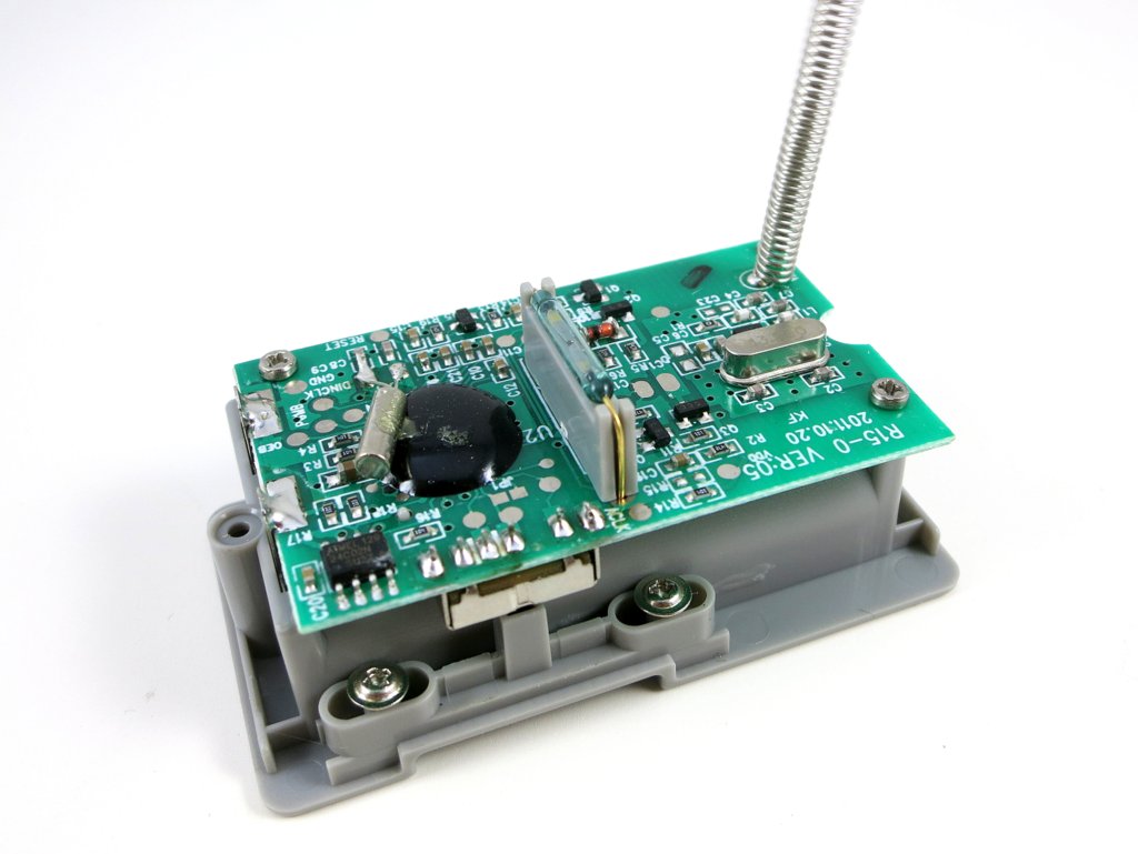
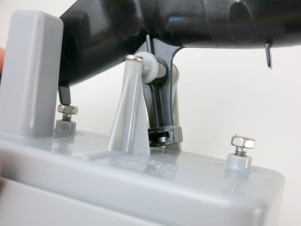
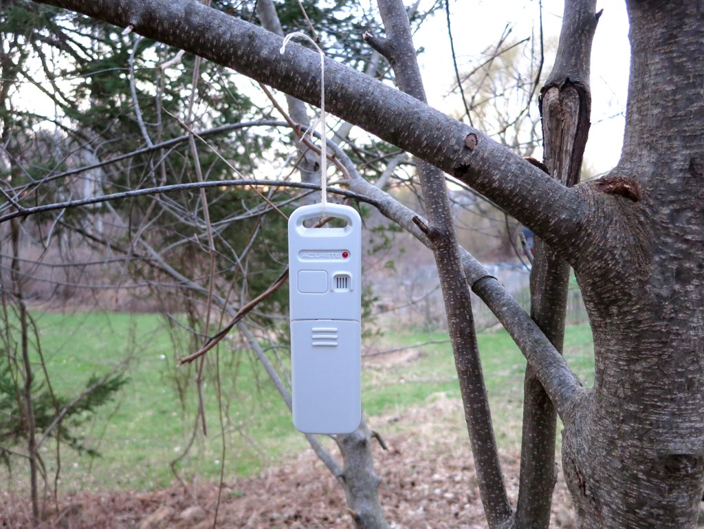
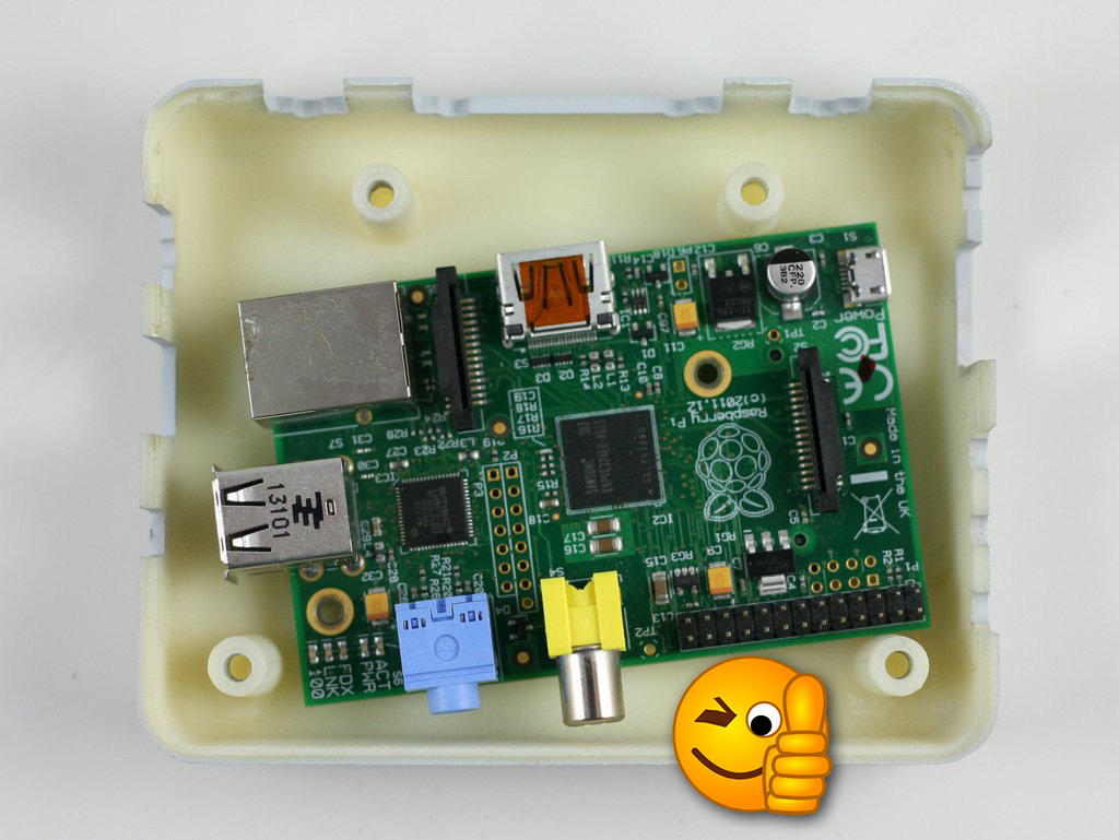
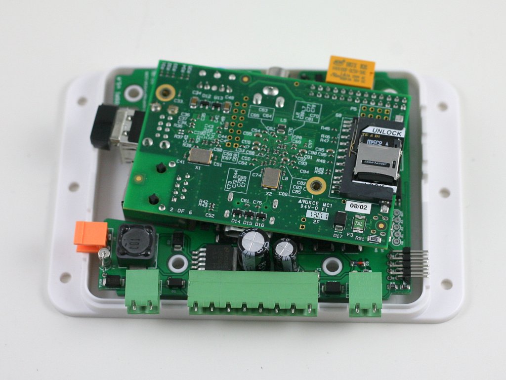
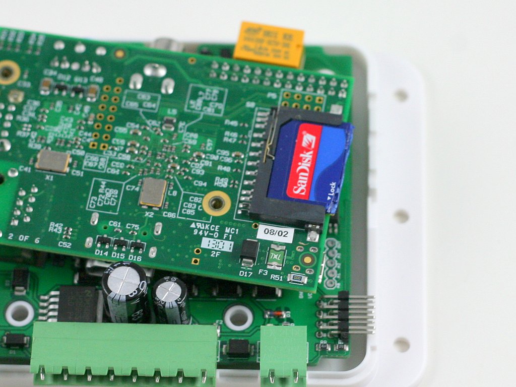
The past week has seen some nice community contributions to SquareWear 2.0. The first is a 3D printed strap-on case designed by Paul Modiano:

Very nice and makes SquareWear truly wearable 🙂 The add-on module in the picture is an ADXL335 accelerometer which takes analog pins A4, A2 and A3. The 3D files can be downloaded from Thingiverse. Thanks Paul for designing this case!

Next is an April fool’s day prank created by Steve Edwards. I don’t have a picture of it, but here is Steve’s description from the comments section:

Great platform for April Fools.

I wrote a sketch that ‘delays’ for 3 hours (to give you a chance to hide the Square and for the victim to fall asleep) and then runs 2 tasks:

1) Every x seconds, beep y tones, of z frequency where x, y, and z are random()ized.

2) Every hour blast out 30 random frequency tones to make sure the victim is awake.

Also, before each tone is played, I check to see if the light sensor is less than 2 so if the victim turns on the lights to look for it, it stops ‘beeping.’

I hid 3 in my son’s room. He didn’t think it was so funny 🙂

Sounds like a fun gadget to annoy someone 🙂

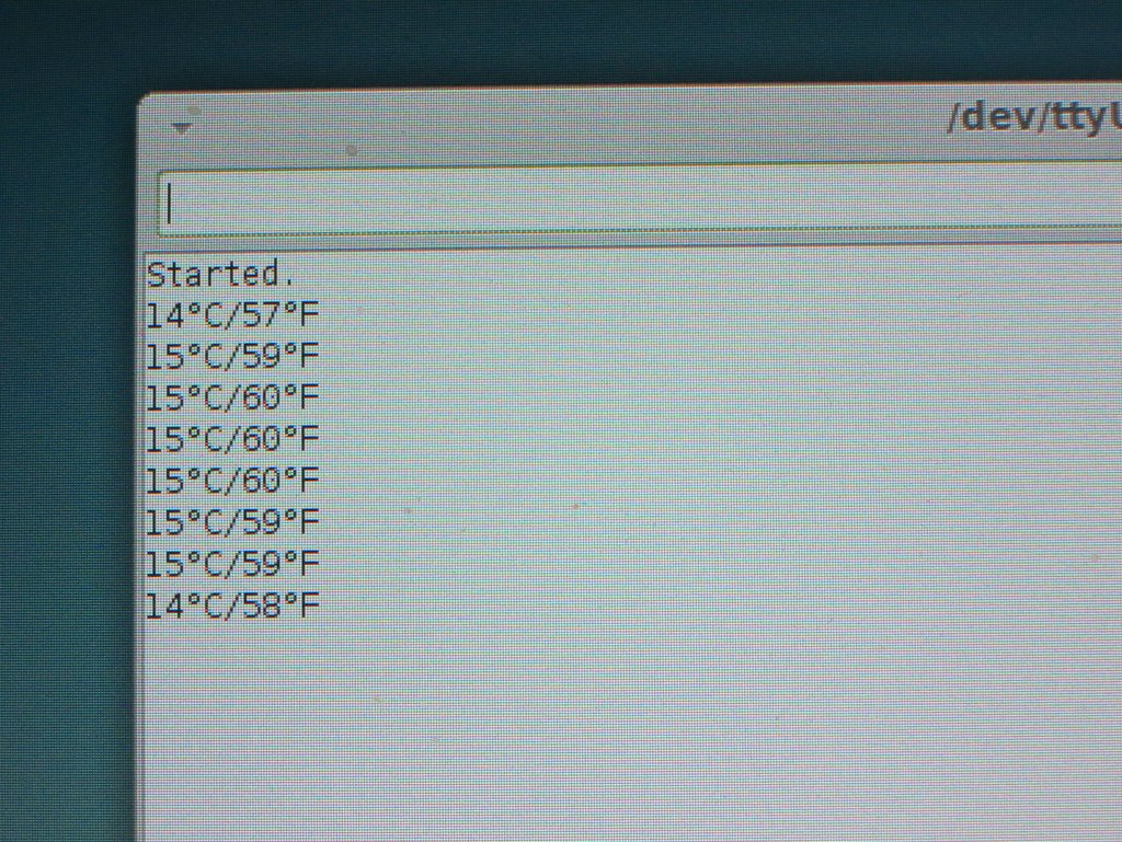
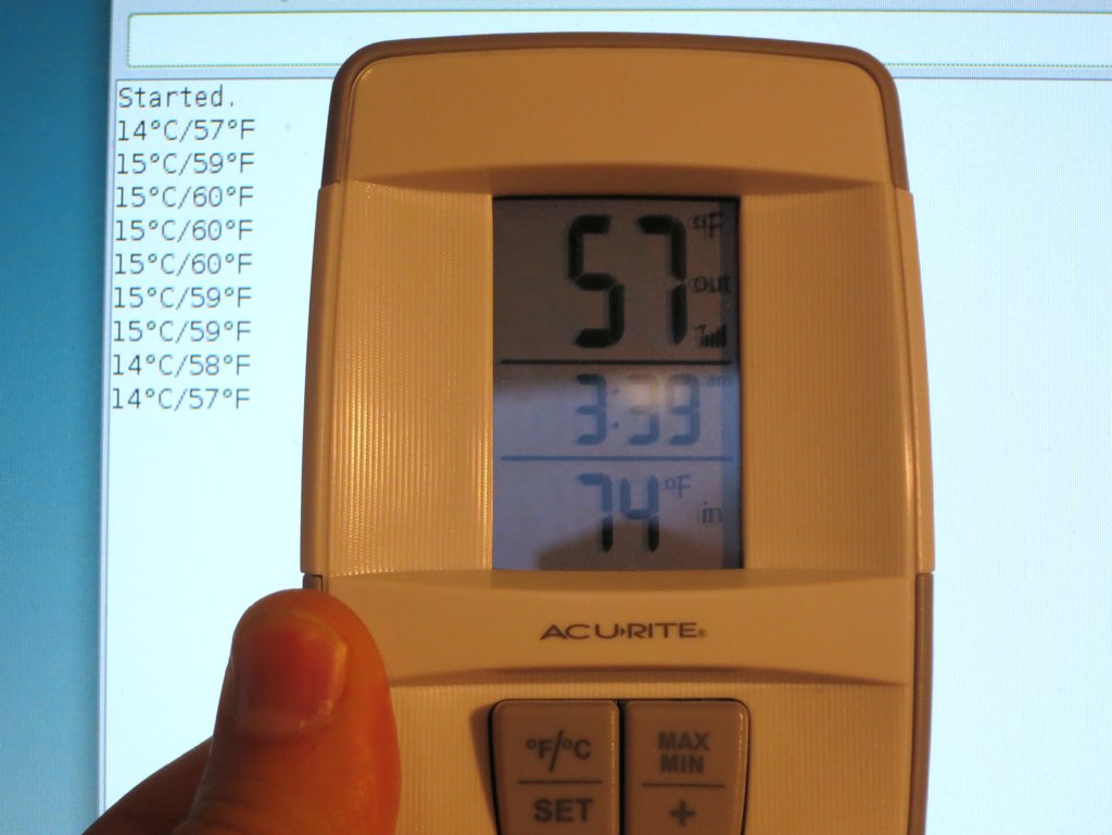
I also got an email from Pete Metcalfe who wrote a temperature display demo using SquareWear 2 and the chainable LED matrix. He made a compact display by creating a new, 3×5 pixel array of numbers. The source code is posted below.

sqrwear_tempdisplay

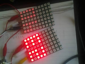
I am so glad to see SquareWear 2.0 being gradually picked up by the community, and the interesting applications created and shared by users. More to come later!


// Pete's temperature display demo
void loop(){
float temp = (float)analogRead(PINTEMP);
temp = (temp * 3.3 / 1024 - 0.5) / 0.01; // MCP9700.MCP9700A
clearStrip();
// define a 3x5 pixel array
int nums[10][13] = {
{ 0, 1, 2, 7, 9,14,16,21,23,28,29,30,30}, //0
{ 1, 8, 9,15,22,28,29,30,30,30,30,30,30}, //1
{ 0, 1, 2, 7,14,15,16,23,28,29,30,30,30}, //2
{ 0, 1, 2, 7,14,15,16,21,28,29,30,30,30}, //3
{ 0, 2, 7, 9,14,15,16,21,28,28,28,28,28}, //4
{ 0, 1, 2, 9,14,15,16,21,28,29,30,30,30}, //5
{ 2, 9,14,15,16,21,23,28,29,30,30,30,30}, //6
{ 0, 1, 2, 7,14,21,28,28,28,28,28,28,28}, //7
{ 0, 1, 2, 7, 9,14,15,16,21,23,28,29,30}, //8
{ 0, 1, 2, 7, 9,14,15,16,21,28,28,28,28} //9
};
int dig10 = int(temp/10);
int dig1 = temp - (dig10*10);
for(int i = 0; i < 13 ; i++){ strip.setPixelColor((nums[dig10][i]+4),0,0,255); } for(int i = 0; i < 13 ; i++){ strip.setPixelColor((nums[dig1][i]),0,0,255); } strip.show(); delay(2000); } void clearStrip(){ for(int i = 0; i < strip.numPixels(); i++){ strip.setPixelColor(i,0,0,0); } strip.show(); }