Reverse Engineer a Cheap Wireless Soil Moisture Sensor

At the Maker Faire this year I got lots of questions about soil moisture sensors, which I knew little about. So I started seriously researching the subject. I found a few different soil sensors, learned about their principles, and also learned about how to make my own. In this blog post, I will talk about a cheap wireless soil moisture sensor I found on Amazon.com for about $10, and how to use an Arduino or Raspberry Pi to decode the signal from the sensor, so you can use it directly in your own garden projects.

What is this?
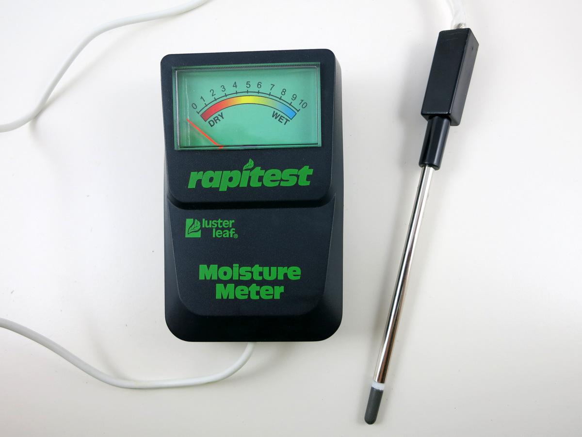
A soil moisture sensor (or meter) measures the water content in soil. With it, you can easily tell when the soil needs more water or when it’s over-watered. The simplest soil sensor doesn’t even need battery. For example, this Rapitest Soil Meter, which I bought a few years ago, consists of simply a probe and a volt meter panel. The way it works is by using the Galvanic cell principle — essentially how a lemon battery or potato battery works. The probe is made of two electrodes of different metals. In the left picture below, the tip (dark silver color) is made of one type of metal (likely zinc), and the rest of the probe is made of another type of metal (likely copper, steel, or aluminum). When the probe is inserted into soil, it generates a small amount of voltage (typically a few hundred milli-volts to a couple of volts). The more water in the soil, the higher the generated voltage. This meter is pretty easy to use manually; but to automate the reading you need a microcontroller to read the value.

Resistive Soil Moisture Sensor
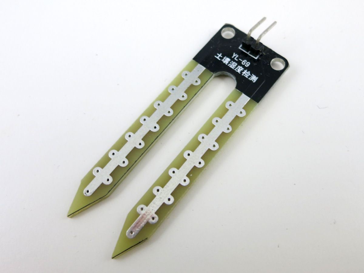
Another type of simple soil sensor is a resistive sensor (picture on the right above). It’s made of two exposed electrodes, and uses the fact that the more water the soil contains, the lower the resistance between the two electrodes. The resistance can be measured using a simple voltage dividier and an analog pin. While it’s very simple to construct, resistive sensors are not extremely reliable, because the exposed electrodes can degrade and get oxidized over time.

Capacitive Soil Moisture Sensor
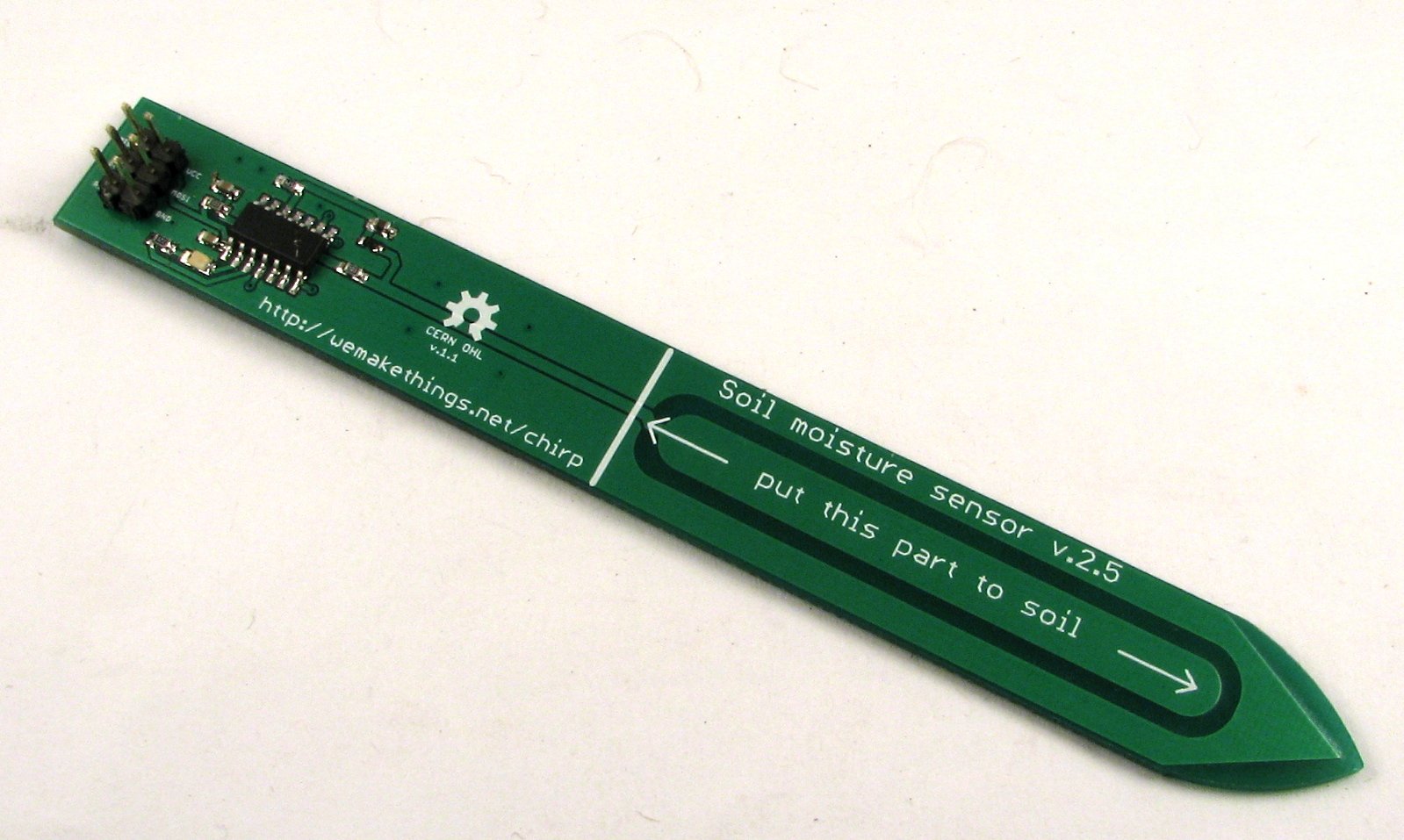
Capativie soil sensors are also made of two electrodes, but insulated (i.e. not exposed). The two electrodes, together with the soil as a dielectric material, form a capacitor. The higher the water content, the higher the capacitance. So by measuring the capacitance, we can infer the water content in soil. There are many ways to measure capacitance, for example, by using the capacitor’s reactance to form a voltage divider, similar to the resistor counterpart. Another way is to create an RC oscillator where the frequency is determined by the capacitance. By counting the oscillation frequency, we can calculate the capacitance. You can also measure the capacitance by charging the capacitor and detecting the charge time. The faster it charges, the smaller the capacitance, and vice versa. The Chirp (picture below), which is an open-source capacitive soil sensor, works by sending a square wave to the RC filter, and detecting the peak voltage. The higher the capacitance, the lower the peak voltage. Capacitive sensors are not too difficult to make, and are more reliable than resistive ones, so they are quite popular.

More Complex Soil Sensors
There are other, more complex soil sensors, such as Frequency Domain Reflectometry (FDR), Time Domain Reflectometry (TDR), and neutron sensors. These are more accurate but also will cost a fortunate to make.

Wireless Soil Moisture Sensor
Because soil sensor is usually left outdoors, it’s ideal to have it transmit signals wirelessly. In addition, because soil moisture can vary from spot to spot, it’s a probably good idea to use multiple sensors distributed at different locations to get a good average reading. Wireless would make it more convenient to set up multiple sensors.

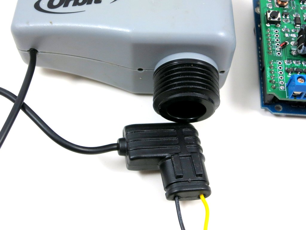
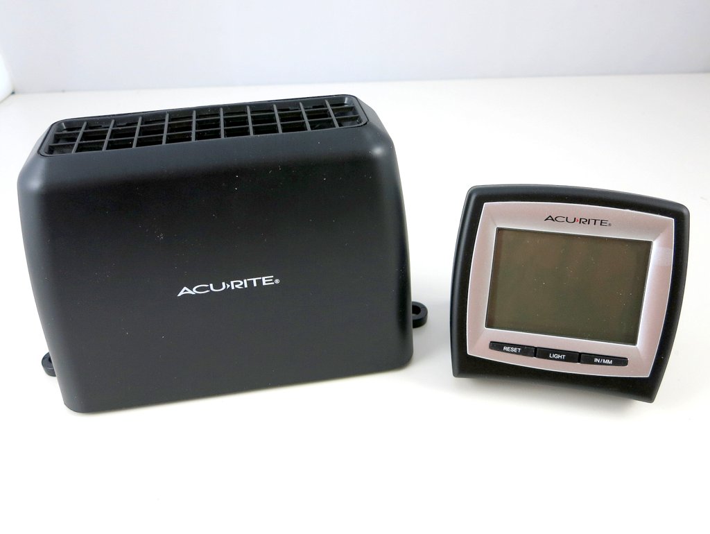
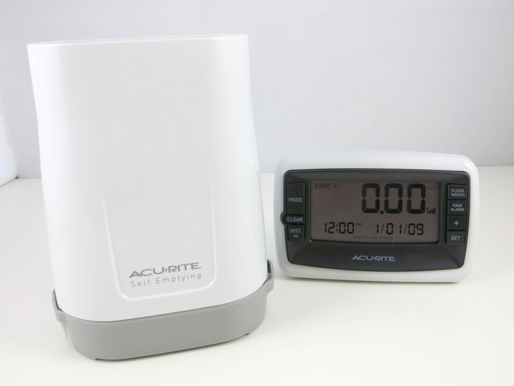
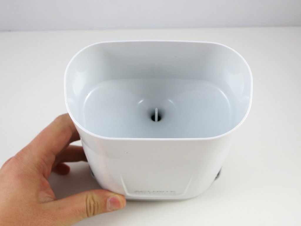
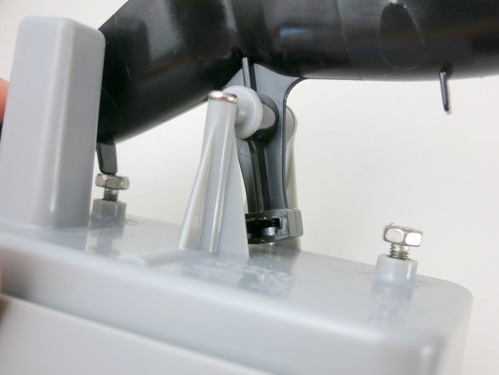
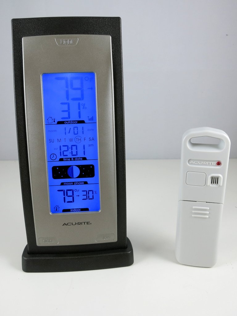
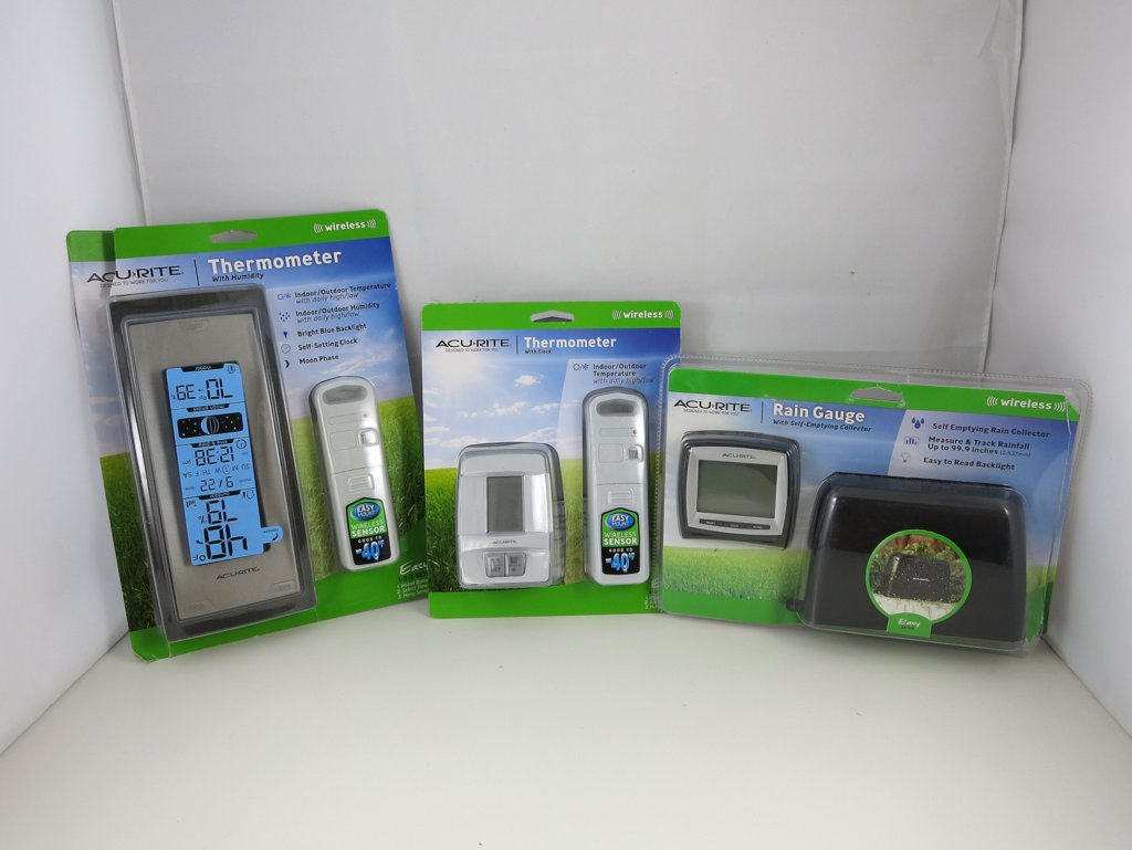
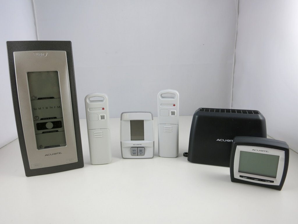
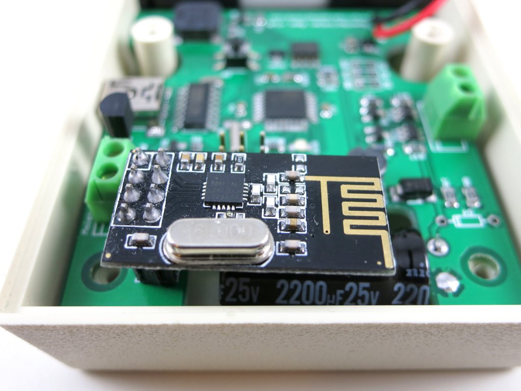
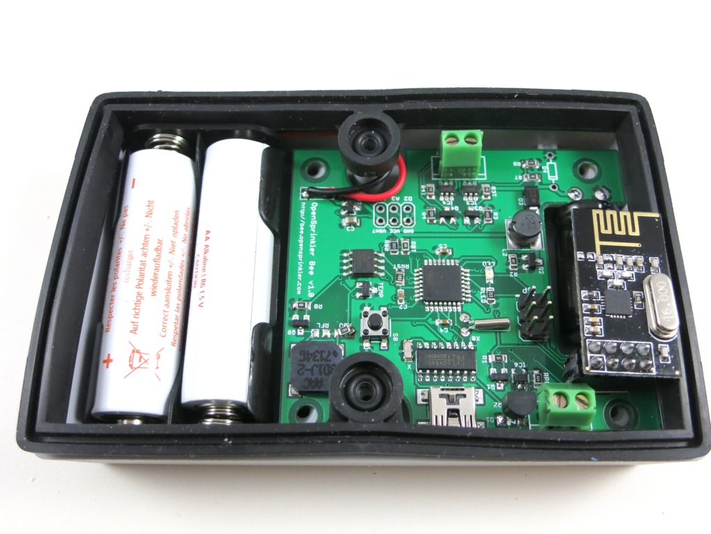
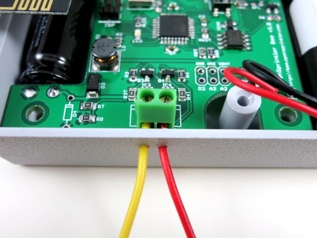
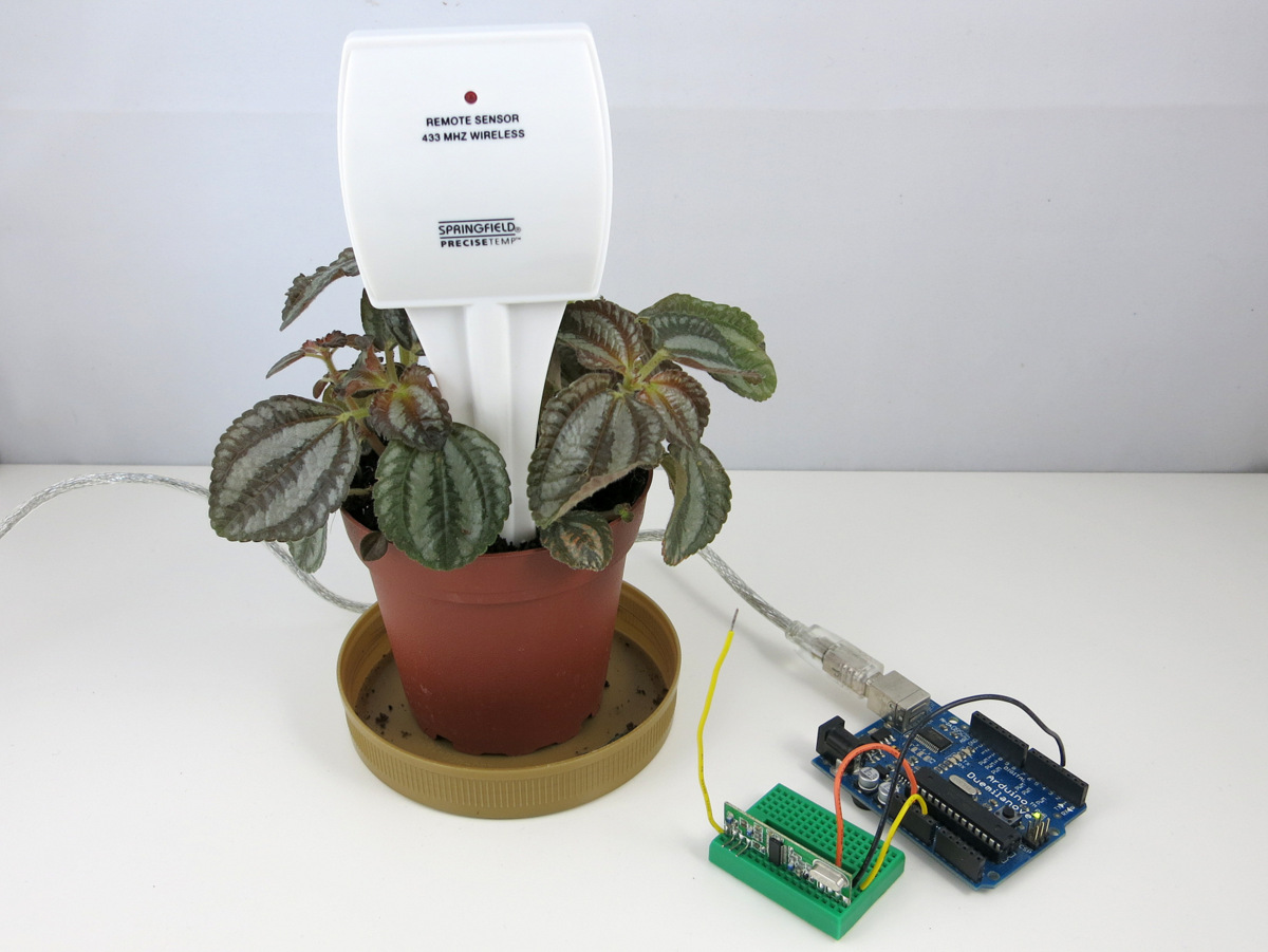
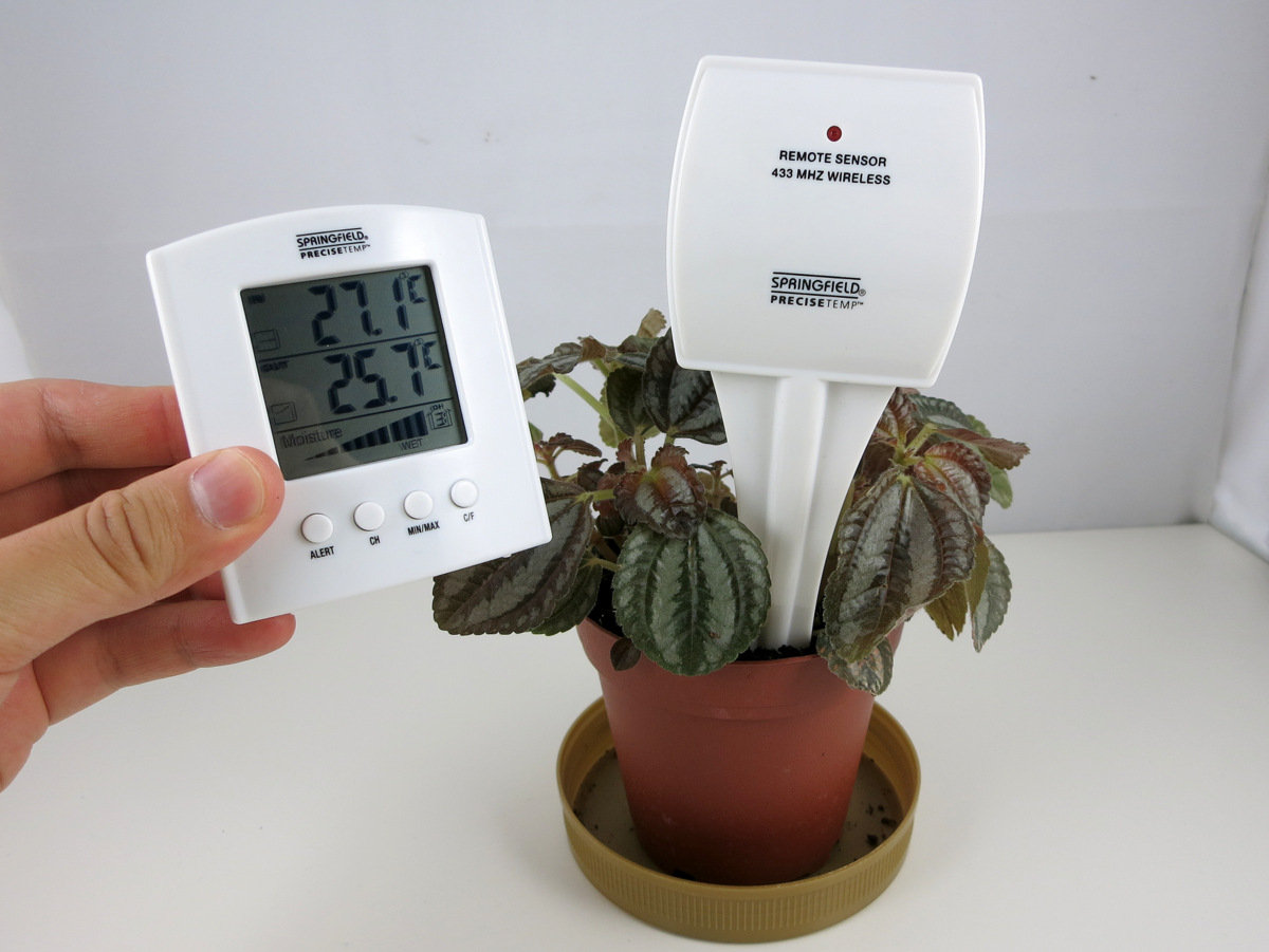
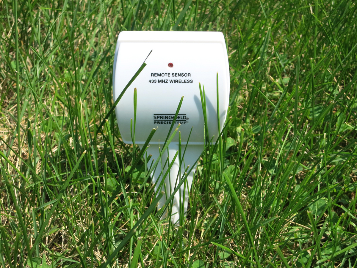
Recently I found this 433MHz wireless soil sensor from Amazon, for only $10, very cheap. It comes with a transmitter unit and a receiver display unit. The transmitter unit has a soil probe. The receiver unit has a LCD — it displays soil moisture level (10 bars) and additionally indoor / outdoor temperature. Let me open up the transmitter to see what’s inside:

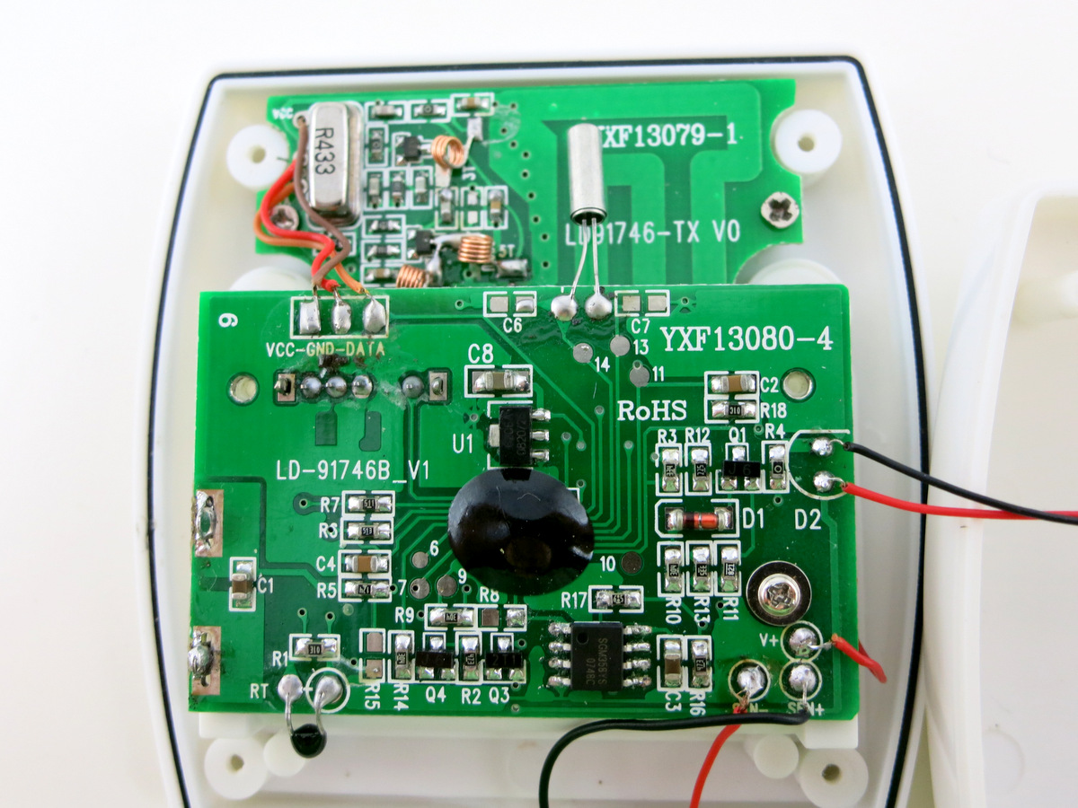
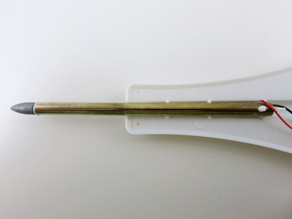
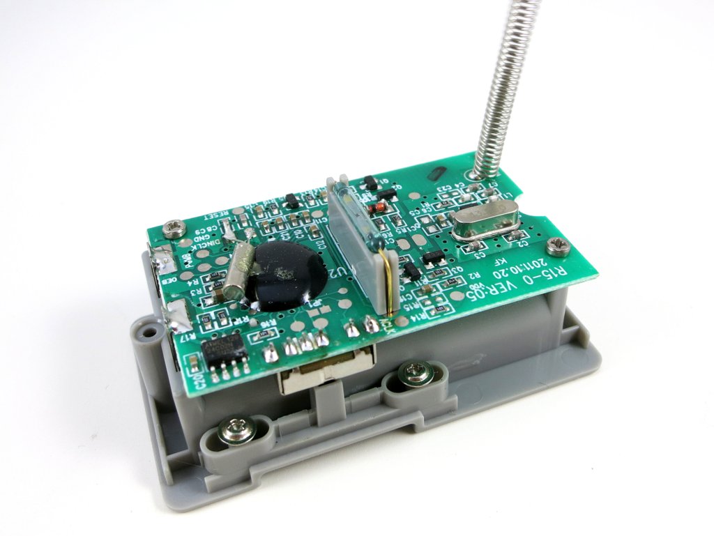
There is a soil probe, a 433MHz transmitter, a microcontroller at the center, a thermistor, and a SGM358 op-amp. Pretty straightforward. The soil probe looks quite similar to the battery-free soil meter probe that I mentioned above. So I am pretty sure this is not a resistive or capacitive probe, but rather a Galvanic probe. Again, the way it works is by outputting a variable voltage depending on the water content in soil. By checking the PCB traces, it looks like the op-amp is configured as a voltage follower, which allows the microcontroller to reliably read the voltage generated by the Galvanic probe.

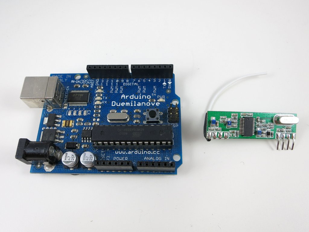
Now we understand the basic principle of the sensor, let’s take a look at the RF signal from the sensor. I’ve done quite a few similar experiments before, so I will just follow the same procedure as described in this post.

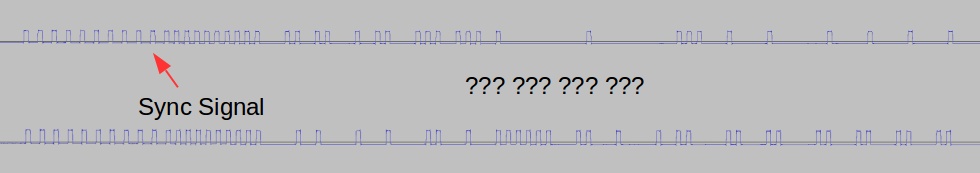
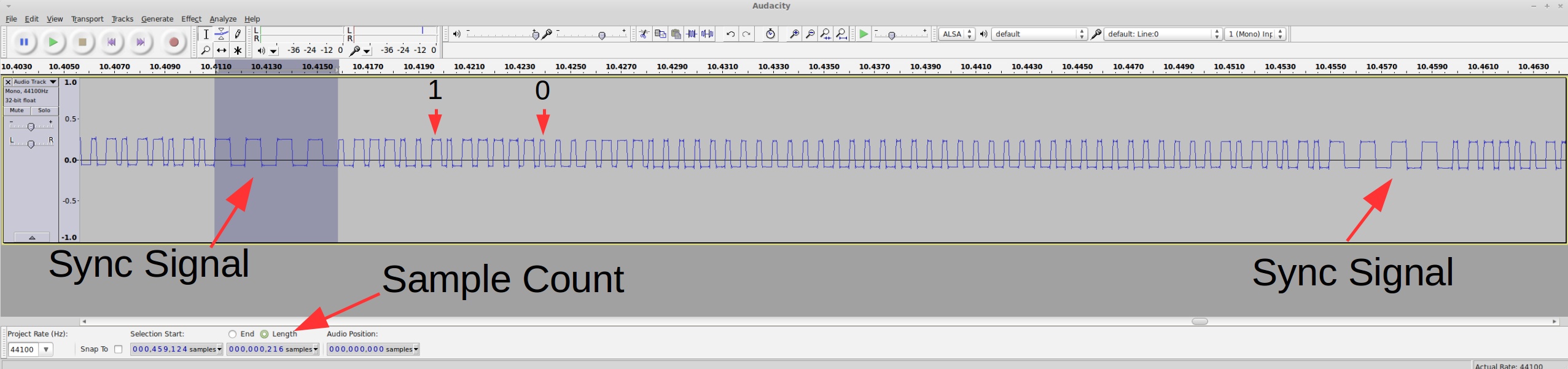
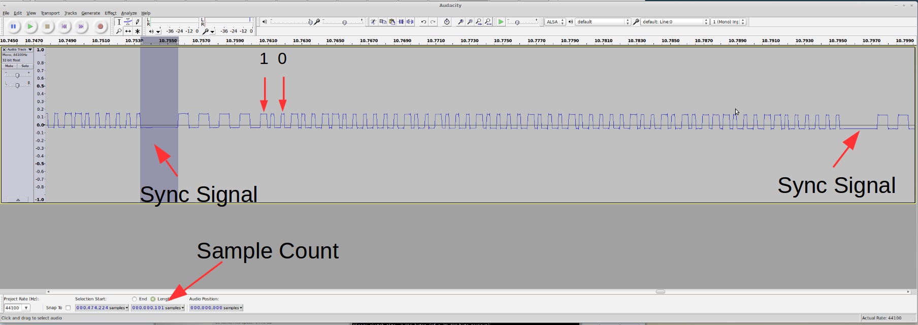
Raw Waveform. To begin, I use a RF sniffing circuit to capture a raw waveform, which looks like this:

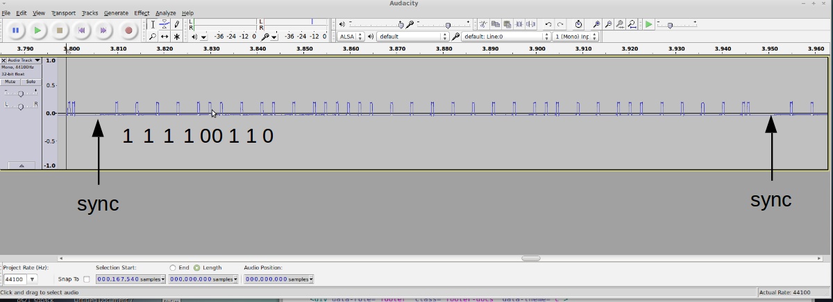
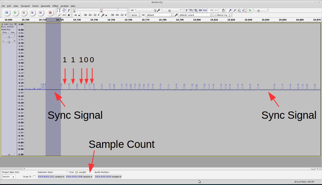
Encoding. Each transmission consists of 8 repetitions. The above shows one repetition: it starts with a sync signal (9000us low); a logic 1 is a impulse (475us) high followed by a 4000us low; a logic 0 is the same impulse high followed by a 2000us low. So the above signal translates to:

11110011 01100000 11111111 00111001 1111

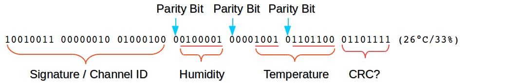
The signal encodes both temperature and soil humidity values. By varying temperature and soil moisture, and observing how the signals change, it’s pretty easy to figure out that the 12 bits colored blue correspond to temperature (10 times Celcius), and the 8 bits colored red corespond to the soil moisture value. The first 12 bits are device signature, which is quite typical in this type of wireless sensors; the last four bits are unclear, but likely some sort of parity checking bits for the preceding four bytes). So the above signal translates to 25.5°C and a soil moisture value of 57.

The display unit shows soil moisture level in 10 bars — 1 to 3 bars are classifed as ‘dry’, 4 to 7 bars are classified as ‘damp’, and above 7 bars are classified as ‘wet’. How does this translate to the soil moisture value? Well empirically (from the data I observed) the dry-damp boundary is around 60, and damp-wet boundary is around 100.

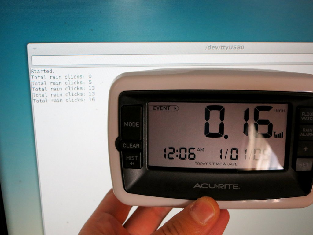
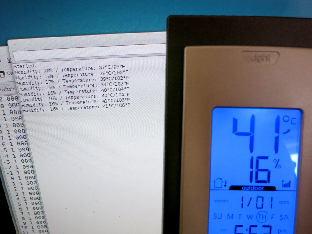
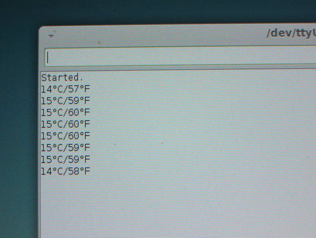
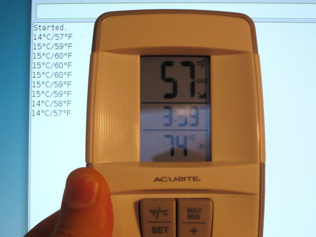
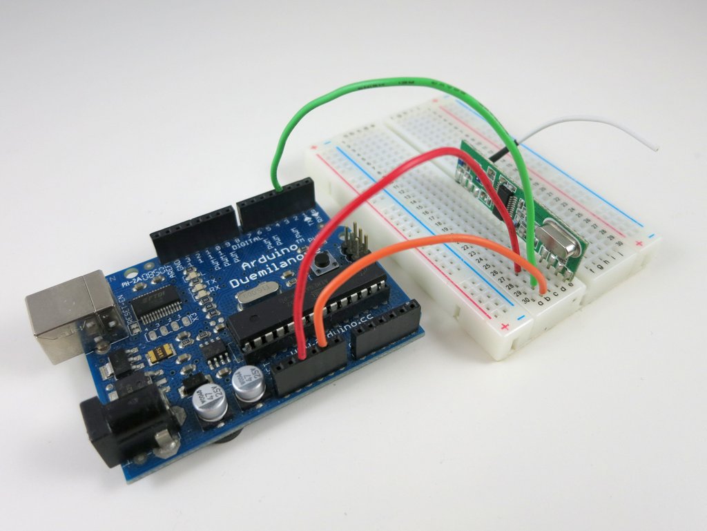
Arduino Program. I next wrote an Arduino program to listen to the sensor and display the soil moisture value and temperature to the serial monitor. For this you will need a 433MHz receiver, and the program below assumes the receiver’s data pin is connected to Arduino digital pin 3. Because the encoding scheme is very similar to a wireless temperature sensor that I’ve analyzed before, I took that program and made very minimal changes and it worked instantly.

Download the Arduino Program for Wireless Soil Moisture Sensor

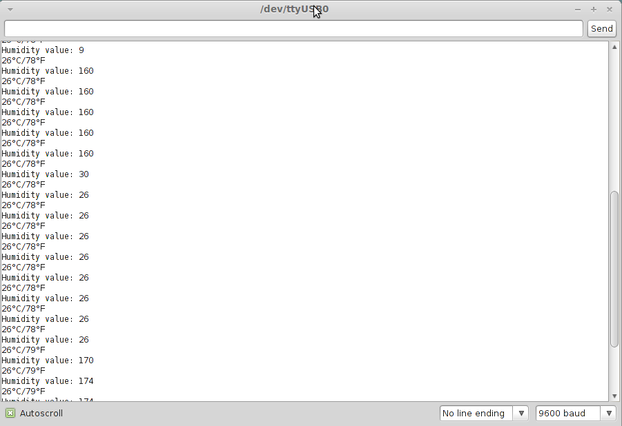
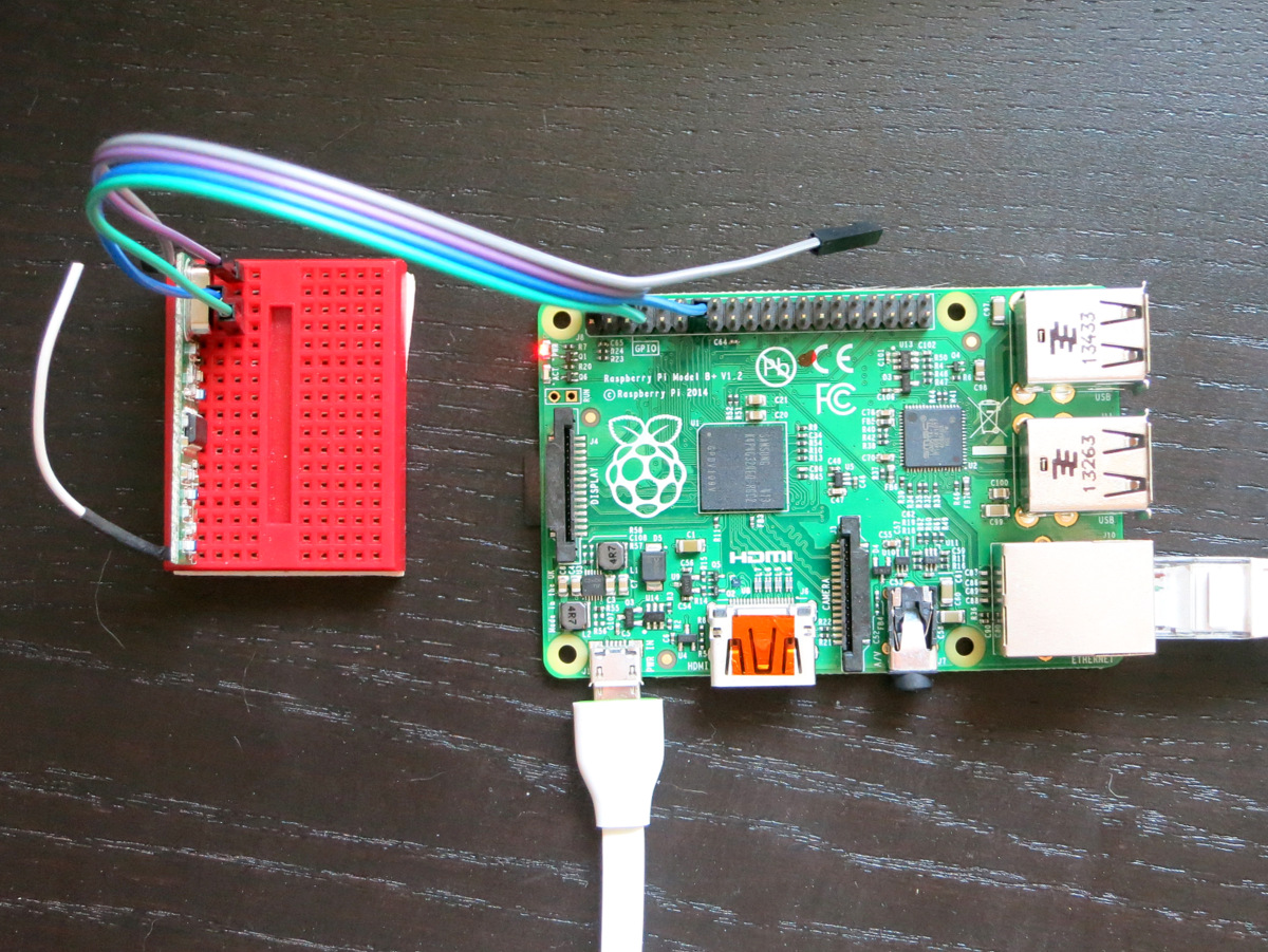
Raspberry Pi Program. By using the wiringPi library, the Arduino code can be easily adapted to Raspberry Pi. The following program uses wiringPi GPIO 2 (P1.13) for data pin.

Download the RPi Program for Wireless Soil Moisture Sensor

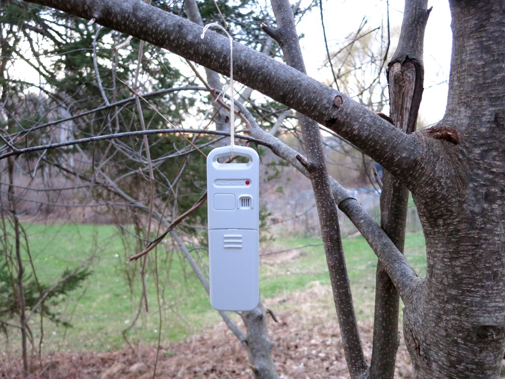
I haven’t done much tests about the transmission range. I’ve put the sensor at various locations on my lawn, and I’ve had no problem receiving signals inside the house. But my lawn is only a quarter acre in size, so it’s not a great test case.

One thing I really liked about using off-the-shelf sensors is that they are cheap and have ready-made waterproof casing. That combined with an Arduino or RPi can enable a lot of home automation projects at low cost.

Announcing OpenSprinkler Bee (OSBee) Arduino Shield v1.0

Update: check out our new standalone OpenSprinkler Bee (OSBee) 2.0 with built-in WiFi and OLED display.

Two months ago, I wrote a blog post about the preview of OpenSprinkler Bee, which is an open-source arduino-based controller for battery-operated sprinkler valves. While that’s still in the development stage, today I am glad to announce that an Arduino shield version of OpenSprinkler Bee is completed and immediately available for purchase at the Rayshobby Shop.

Update: check out our new standalone OpenSprinkler Bee (OSBee) 2.0 with built-in WiFi and OLED display.

So what is this Arduino shield version, and how is this different from other OpenSprinkler prodcuts that we carry? Well, an Arduino shield is a circuit board that you plug into an existing Arduino — it does not have a microcontroller chip itself, but contains additional circuitry that extends the basic functionality of an Arduino. So to use the shield, you will need to provide an existing Arduino board.

How is the OpenSprinkler Bee (OSBee) different from the other OpenSprinkler products? The main difference is that OSBee is designed to work with battery-operated sprinkler valves. These valves internally use a latching solenoid, which only draws power when you open or close the valve, and does not draw power if it remains in the same state. So it’s very efficient and suitable for battery-operated controllers. The other OpenSprinkler products, such as OpenSprinkler 2.1s, DIY 2.1u, OSPi 1.4, OSBo 1.0, are all designed for 24V AC sprinkler valves, which operate on 24V AC and require a power adapter / transformer.

While OSBee shield itself does not have built-in wireless modules, you can stack it with other Arduino shields, such as RF, WiFi, Ethernet shields, to provide web connectivity. The OSBee Arduino library has one example of using the Arduino Ethernet shield with OSBee shield to create a web interface for sprinkler control.

Is there any easy way to tell latching solenoid valves from 24V AC valves? Yes. Latching solenoid valves usually come with a special plug, and the two wires are usually colored differently because the solenoid has polarity. 24V AC valves usually come with just two wires colored in the same way (because AC voltage has no polarity). Here are some examples of latching solenoid valves. Note the special plugs and/or different wire colors.

For valves that come with stripped wires, simply attach them to the screw terminal blocks on OSBee shield. For valves with special plugs, you can cut and strip two pieces of wire (20 to 24 AWG): insert one end of the wire to the plug, and the other end to the screw terminal block.

How to open or close the latching solenoid valve? Electrically, latching solenoid valves have quite low coil resistance (a few ohms). To open the valve, you apply a momentary positive voltage on the coil. The specific voltage depends on the valve specification, but it typically varies between 9V to 22V. To close the valve, just reverse the voltage polarity. The important thing to keep in mind is that the voltage is applied as a pulse — usually 25 to 100 milliseconds. Because the coil resistance is so low, the instantaneous current is very high, up to a few amps. So you can’t apply the voltage continuously (or it will smoke the coil or the power supply!) In addition, it’s better to first build up the voltage into a capacitor, and then dump the charge to the valve from the capaictor.

How to generate such a high voltage from Arduino’s 5V or 3.3V pin? It’s by using a neat circuitry called ‘boost converter‘. The Wikipedia has plenty of information about how it works, but the basic principle is to use a MOSFET switch, an inductor, a diode, and a PWM signal to build up the charge into a capacitor. This way you can generate a high voltage from a low-voltage source such as AA batteries.

How to apply a voltage in both polarities? This is by using another neat circuitry called ‘H-Bridge‘. The H-Bridge is made of four MOSFET switches. By closing the pair of switches in each diagonal direction, you can apply voltage in either positive or negative polarity. Because you also need a state where no voltage is applied on the solenoid, that’s three states in total and hence two microcontroller pins are required to produce three states. Wait, why not directly use two microcontroller pins to apply the voltage? Well, microcontroller pins can neither handle high voltage nor provide high current, so you need MOSFETs to help switch high voltage and high current using only logic signals from the microcontroller.

With all the technical concepts explained, here is the diagram of the various components on the OSBee Sheild:

The shield can switch 4 independent valves / zones. The boosting voltage is software adjustable — anywhere from 9V to 24V. An Arduino library with three demo programs are provided in the OSBee Github repository. For details, please refer to:

OSBee Shield v1.0 User Manual

OSBee Shield v1.0 is now available for purchase at the Rayshobby Shop. Thanks!

SquareWear 2.0 is now available at SeeedStudio.com

This is a quick announcement that SquareWear 2.0 is now available for purchase at SeeedStudio.com.

This is great news for customers living outside of the US, because SeeedStudio offers excellent and low-cost international shipping options.

Reverse Engineer Wireless Temperature / Humidity / Rain Sensors — Part 3

Continuing from Part 1 and Part 2, this is the third and last post about how I reverse engineered a few off-the-shelf wireless temperature, humidity, and rain sensors, and used an Arduino to listen to and decode the sensor data. Update: RPi is also supported now! Check the provided programs at the end of this post.

Wireless Rain Sensor

Raw Waveform. There are several different wireless rain sensors on the market. My first target was an Acu-Rite 00875W rain gauge. I bought it two years ago and I don’t know if it’s still available now. This sensor turns out to be a huge pain. The main problem is that I can’t even register a consistent reading at 0 — every time I pop in the battery, I get a different signal that seems to have nothing to do with the previous readings. Also, the 0/1 bit patterns are completely unclear from the captured waveform — there are at least 4 or 5 different wavelengths. Here are two examples of the captured waveforms. They look nothing alike, even though both were captured right after the batteries are popped in and no rain has been detected.

After pulling my hair for a couple of days and finding no clue at all, I decided to give it up and try a different model. This time I bought an Acu-Rite 00899 wireless rain gauge. It’s probably worth explaining at first how the rain gauge works, because it’s quite a clever design. The outside of the transmitter unit looks like a bucket. Underneath the bucket is a plastic seesaw which swings left and right. Basically the rain water drains through the bucket hole onto the seesaw, and creates some motion to be detected.

At the bottom of the assembly is the battery compartment. Remove some tiny screws, the transmitter circuit is finally revealed. At the center is a reed switch, which is normally open but will close if there is a magnet nearby. It is very sensitive to magnetism. So where is the magnet? It’s on the bottom of the seesaw. The way this works is quite neat: the seesaw swings left and right, every time the magnet passes by the reed switch, it triggers a click. By detecting how many clicks there are within a given time, we know how heavy the rain is. Clever!

So let’s see if this rain gauge is easier to tackle. Following the same procedure as before, pop in the battery, power on the RF sniffing circuit, and launch the Audacity recording software, I got a waveform like the one shown in the image below.

Cool, this looks a lot better. I also made sure every time I pop in the battery I get the same waveform. So what patterns do I see here?

Each transmission consists of 3 repetitions of the same signal.
Every two repetitions are separated by a sync signal defined as 4 squarewaves of roughly 1.2ms wavelength.
The bit patterns are: logic 1 is defined by a constant high of 400us followed by a constant low of 200us; and logic 0 is defined by a constant high of 225us followed by a constant low of 400us.

The sync signal is actually very similar to the humidity/temperature sensor I described in the Part 2. The difference is that there is no 2.25ms constant low preceding the 4 squarewaves.

Given the timing data, here is the Arduino program to convert this signal into bits:

Download the Arduino Program for Sniffing Bits (rain gauge version)

Collect and Analyze Data. The transmitter sends a signal every two minutes, so it’s quite annoying that I had to wait two minutes for every reading. To create variations in data, I simply move the seesaw manually. This way I can precisely control how many clicks occurred between two readings. Here is a list of readings I captured. The numbers in the parentheses are the number of clicks since last reading, and the total number of clicks since the program started.

01110010 11111000 11110000 00000000 00000000 00000000 00000000 01011010 (0 / 0 total) 01110010 11111000 11110000 00000000 00000000 00000000 10000001 11011011 (1 / 1 total) 01110010 11111000 11110000 00000000 00000000 00000000 10000010 11011100 (1 / 2 total) 01110010 11111000 11110000 00000000 00000000 00000000 00000011 01011101 (1 / 3 total) 01110010 11111000 11110000 00000000 00000000 00000000 10000100 11011110 (1 / 4 total) 01110010 11111000 11110000 00000000 00000000 00000000 10000111 11100001 (3 / 7 total) 01110010 11111000 11110000 00000000 00000000 00000000 10001101 11100111 (6 / 13 total)
The encoding scheme is quite obvious: the first three bytes are the signature / device ID; the next 4 bytes record the total number of clicks since the transmitter is powered on. The leading bit of each byte is a parity bit (thanks to the lesson I learned from Part 2!) The last byte is for error checking.

This time I looked at the error checking byte more carefully, and noticed some interesting patterns. For example, everything else being the same, the change in its first bit matches the change of the first bit in the second to last byte. This suggest that perhaps the last byte is a parity byte — specifically, bit 0 is the parity of the first bits in all the preceding 7 bytes, and bit 1 is the parity of the second bit in all the preceding 7 bytes and so on. Just eyeballing the numbers, I believe this looks correct.

I felt quite happy that I made the right choice to abandon the first rain gauge which proved to be too difficult to solve. Well, dodging the challenge is not generally recommended, but in this particular case, I have no regret 🙂

Arduino Program and Validation. Here is the Arduino program that listens to the rain gauge and displays the number of clicks onto the serial monitor. The numbers have been validated with the display unit.

Download the Arduino Program for Wireless Rain Gauge

Update: the code is adapted to RPi as well, using wiringPi. The code below uses wiringPi GPIO 2 (P1.13) for data pin.

Download the Raspberry Pi Program for Wireless Rain Gauge

This concludes the three-part series. If you have comments / questions / suggestions, please feel free to leave them below. Thanks!

New: continue to Part 4, wireless soil moisture sensor.

Reverse Engineer Wireless Temperature / Humidity / Rain Sensors — Part 2

Continuing from Part 1, this is the second post about how I reverse engineered a few off-the-shelf wireless temperature, humidity, and rain sensors, and used an Arduino to listen to and decode the sensor data. Update: RPi is also supported now! Check the provided programs at the end of this post.

Wireless Humidity / Temperature Sensor

Raw Waveform. The second sensor to tackle is the Acu-Rite 00592W3 humidity / temperature sensor. This one transmits not only temperature but also humidity values. The display unit is a lot larger and looks cooler than the previous (temperature-only) one. Cool, time to get hands dirty. Following the same procedure as before, pop in the battery, power on the RF sniffing circuit, and launch the Audacity recording software, I got a waveform like the one shown on the right image below.

This looks a whole lot longer than before. But the patterns are still quite clear:

Each transmission consists of 3 repetitions of the same signal.
Every two repetitions are separated by a sync signal defined as a constant low of 2.25ms (about 100 samples @ 44.1kHz sample rate). This is followed by 4 squarewaves of roughly 1.2ms wavelength.
The bit patterns are also clear as there are only two types of patterns: logic 1 is defined by a constant high of 400us followed by a constant low of 225us; and logic 0 is defined by a constant high of 250us followed by a constant low of 400us.

Given the timing data, I quickly modified the Arduino program to convert this signal into bits. The only changes are how the sync signal is detected, and how the bit 1 and 0’s are defined.

Download the Arduino Program for Sniffing Bits (humidity/temperature sensor version)

Collect and Analyze Data. I collected a few groups of data under different humidity and temperature conditions, and recorded the reference values shown on th

Download the Arduino Program for Wireless Rain Gauge

e display unit. Given my experience with the first temperature sensor, I set the display unit to show temperature in Celsius, to save myself the trouble of doing the conversion. Here is a selected list of the data:

10010011 00000010 01000100 00100010 00001001 10111110 11000010 (21°C/34%) 10010011 00000010 01000100 00100010 00001001 11000101 11001001 (22°C/34%) 10010011 00000010 01000100 10100011 00001001 11011000 01011101 (24°C/35%) 10010011 00000010 01000100 00100010 00001001 01100101 01101001 (25°C/34%) 10010011 00000010 01000100 00100001 00001001 01101100 01101111 (26°C/33%) 10010011 00000010 01000100 10100000 00001001 11110011 01110101 (26°C/32%) 10010011 00000010 01000100 10100000 00001001 11111001 01111011 (27°C/32%) 10010011 00000010 01000100 10011111 00001010 10000001 00000011 (28°C/31%) 10010011 00000010 01000100 00011110 00001010 10010011 10010100 (29°C/30%) 10010011 00000010 01000100 00010100 00001010 11001001 11000000 (35°C/20%) 10010011 00000010 01000100 10010000 00001010 11010111 01001010 (36°C/16%)

Again, I grouped the data into bits of 8 to make it easy to see the byte values. The first three bytes are the same. Those are probably the signature / channel ID; the fourth byte is clearly correlated with the humidity — if you pick two lines with the same humidity value, the fourth byte is always the same. On close examination, the lowest 7 bits of that byte converts exactly to the decimal value of the humidity. To make it clear, I picked out the fourth byte, and wrote them down together with the reference humidity below:
0 0100010 (34%) 0 0100010 (34%) 1 0100011 (35%) 0 0100010 (34%) 0 0100001 (33%) 1 0100000 (32%) 1 0100000 (32%) 1 0011111 (31%) 0 0011110 (30%) 0 0010100 (20%) 1 0010000 (16%)
Aha, one puzzle is now solved. Not sure what the leading bit is (this will be revealed later), but we can move on to the next puzzle — temperature. Clearly the temperature has to do with only the last three bytes. So let me re-list them below with the reference temperature:
00001001 10111110 11000010 (21°C) 00001001 11000101 11001001 (22°C) 00001001 11011000 01011101 (24°C) 00001001 01100101 01101001 (25°C) 00001001 01101100 01101111 (26°C) 00001001 11110011 01110101 (26°C) 00001001 11111001 01111011 (27°C) 00001010 10000001 00000011 (28°C) 00001010 10010011 10010100 (29°C) 00001010 11001001 11000000 (35°C) 00001010 11010111 01001010 (36°C)
Because the data was recorded as the temperature went up, the first byte is clearly showing the right trend: it goes up as the temperature rises. These are probably the most significant 4 bits. The next byte is not very clear at all: sometimes it goes up, sometimes it goes down. What’s happening here? The last byte is even more elusive: but given my experience with the first temperature sensor, this is probably some sort of error checking code, so let me put it aside for now.

To figure out what’s happening with the second byte, I needed more data. Using my old friends hair blower and fridge, I recorded a larger set of data, and here they are:
00000110 11101011 11011100 (-13°C) 00000110 11111001 11110000 (-12°C) -------- -------- -------- -------- 10000111 00000000 01111000 (-11°C) 10000111 00110101 10110010 (-6°C) 10000111 11010001 01001110 (-3°C) 10000111 11011011 01011000 (-2°C) 10000111 01011111 11011100 (-1°C) 10000111 01101111 11101101 ( 0°C) 10000111 11111001 11111000 ( 1°C) -------- -------- -------- -------- 10001000 00000011 00000011 ( 2°C) 10001000 00010100 10010011 ( 4°C) 10001000 01000001 00111110 ( 8°C) 10001000 11110011 11100100 (13°C) 10001000 01111101 01101110 (14°C) -------- -------- -------- -------- 00001001 00000110 01111000 (15°C) 00001001 00001111 10000001 (16°C) 00001001 00100010 10010100 (18°C) 00001001 11011110 01011111 (24°C) 00001001 11111100 11111001 (27°C) -------- -------- -------- -------- 00001010 00000011 00000001 (28°C) 00001010 00001111 00001101 (29°C) 00001010 11010001 01000100 (36°C) 00001010 01100110 11011001 (38°C) 00001010 11111111 01110010 (40°C) -------- -------- -------- -------- 10001011 10001110 10000010 (42°C) 10001011 00011101 00010001 (43°C) 10001011 01010011 01000111 (49°C) 10001011 01111000 01101100 (52°C) -------- -------- -------- -------- 00001100 10000001 11110110 (53°C)

The second byte still doesn’t show any clear trend; but the first byte is still well behaved: it consistently increments as the temperature rises. That’s re-assuring. I then noticed something very interesting, and that’s why I used dotted lines to separate the data: each dotted line marks where the first byte increments by 1. If you look at the temperature where these changes occur, there is an interesting pattern: the change occurs roughly every 12 degree Celsius.

From my experience with the first temperature sensor, I know that it’s likely the data reflects 10 times the Celsius, so that means the change occurs at about every 120. This is very close to 128. If this is the case, then the lowest bit of the first byte must be the 8-th bit of the actual data (that’s how one bit of increment corresponds to a change of 128), and thus there must be 7 least significant bits following it! Could that be from the second byte?

After staring at the data for a while, I see a path now: if you put together the lowest 4 bits of the first byte and the lowest 7 bits of the second byte, into a 11-bit binary number, this number consistently rises with the temperature. Aha, let me wrote them down here:
0110 1101011 (-13°C) -> 875 => -14.9 0110 1111001 (-12°C) -> 889 => -13.5 0111 0000000 (-11°C) -> 896 => -12.8 0111 0110101 (-6°C) -> 949 => -7.5 0111 1010001 (-3°C) -> 977 => -4.7 0111 1011011 (-2°C) -> 987 => -3.7 0111 1011111 (-1°C) -> 991 => -3.3 0111 1101111 ( 0°C) -> 1007 => -1.7 0111 1111001 ( 1°C) -> 1017 => -0.7 1000 0000011 ( 2°C) -> 1027 => 0.3 1000 0010100 ( 4°C) -> 1044 => 2 1000 1000001 ( 8°C) -> 1089 => 6.5 1000 1110011 (13°C) -> 1139 => 11.5 1000 1111101 (14°C) -> 1149 => 12.5 1001 0000110 (15°C) -> 1158 => 13.4 1001 0001111 (16°C) -> 1167 => 14.3 1001 0100010 (18°C) -> 1186 => 16.2 1001 1011110 (24°C) -> 1246 => 22.2 1001 1111100 (27°C) -> 1276 => 25.2 1010 0000011 (28°C) -> 1283 => 25.9 1010 0001111 (29°C) -> 1295 => 27.1 1010 1010001 (36°C) -> 1361 => 33.7 1010 1100110 (38°C) -> 1382 => 35.8 1010 1111111 (40°C) -> 1407 => 38.3 1011 0001110 (42°C) -> 1422 => 39.8 1011 0011101 (43°C) -> 1437 => 41.3 1011 1010011 (49°C) -> 1491 => 46.7 1011 1111000 (52°C) -> 1528 => 50.4 1100 0000001 (53°C) -> 1537 => 51.3
The single arrow points to the decimal value of the 11-bit number. There is obviously an offset of 1024, so I subtracted the value by 1024 and then divided it by 10. The result is shown following the double arrow.

Now we are almost done. If you compare the result with the reference temperature, there is still some difference, like a 1.6 to 1.9 degree constant shift. This is probably due to calibration. The shift seems consistent, so I picked 1.9 as an empirical number. Putting everything together, the temperature is calculated as: [(11-bit number – 1024) / 10 + 1.9] rounded to the nearest integer.

Parity Checking Bit. At this point you have probably already figured out about the mysterious leading bit (which I ignored above). It is a parity bit — it shows if there are an odd or even number of 1’s in the remaining 7 bits. It’s the simplest form of error detection. Because the first temperature sensor I worked with did not have a parity bit, I didn’t think about it immediately. It’s only after I figured out about the temperature encoding scheme that I came to realize the leading bit must be used for error checking. Here is a summary of the encoding scheme:

At this point, the last byte is still a mystery — as I said, it’s likely some sort of CRC checking code. Perhaps the experts can shed some light here?

Arduino Program and Validation. It’s now time for the final test. Here is the Arduino program that listens to the transmitter and displays the humidity / temperature value to the serial monitor.

Download the Arduino Program for Wireless Humidity/Temperature Sensor

Update: the code is adapted to RPi as well, using wiringPi. The code below uses wiringPi GPIO 2 (P1.13) for data pin.

Download the Raspberry Pi Program for Wireless Humidity/Temperature Sensor

The result matches the display unit quite well. Cool. Mission accomplished!

Continue to Part 3 and Part 4, or Back to Part 1.

Reverse Engineer Wireless Temperature / Humidity / Rain Sensors — Part 1

In this and the next ~~two~~ three blog posts (Part 2, Part 3, and Part 4), I will describe how I reverse engineered a few off-the-shelf wireless temperature, humidity, and rain sensors, and used an Arduino (Update: RPi is also supported now!) to listen to and decode the sensor data. This has been a really fun journey and I will document the process as thoroughly as I can. Because there are lots of details, I don’t want to jam everything into a single post, so I have split the whole story into three posts. The Arduino and RPi programs are provided at the end of each post.

Introduction

The first question to ask is always: why am I doing this? Well, for good reasons: these off-the-shelf sensors are cheap, well-built, outdoor-proof, battery-driven and power efficient. If your project needs local weather data and you don’t want to spend time building your own transmitter units (which would bring up a whole bunch of engineering issues), these cheap sensors are the way to go. My original plan was to make use of the sensor data for sprinkler control systems. I actually set this as my next challenge to tackle in a blog post I wrote two years ago. It’s a shame that I lost track of it since then. But hey, two years later, I finally finished it. Better late than never!

Here are the three sensors that I gathered and will use as examples in the following. They all work in the 433MHz frequency band.

Disclaimer: I am not associated with Acu-Rite in any ways, I just picked these sensors because they are common in retail stores.

Preparation

The tools involved are quite simple: I used an Arduino and a 433MHz receiver. You should use the superheterodyne type of receiver as it has very good signal-to-noise-ratio. The super-regenerative type is too noisy and will only work in short range.

Also, to obtain an initial waveform in order to bootstrap the process, I used a RF sniffing circuit from my previous blog post (about interfacing with remote power sockets), a PC with line-in port, a 3.5mm audio cable, and the free Audacity software. If you don’t have a PC with line-in port (most laptops these days don’t have), you can buy a USB sound card which has line-in port.

Wireless Temperature Sensor

Raw Waveform. The temperature sensor is the simplest, so let’s take it down first. What I have at hand is an Acu-Rite 00782W3 indoor/outdoor temperature sensor. The package includes a receiver display unit, and a transmitter which sends a temperature reading every 1 to 2 minutes. Pop in the battery, power on the RF sniffing circuit, and launch the Audacity recording software, I got a waveform like the one shown on the right image below.

By carefully looking at the waveform, I found the following patterns:

Each transmission consists of 8 repetitions of the same signal.
Every two repetitions are separated by a constant low sync signal that’s roughly 400 samples (in Audacity you can select a region and see the sample count). Given that the sampling rate is 44.1kHz, this is roughly 9.0ms (400 / 44.1 = 9.07).
The bit patterns are pretty clear: logic 1 is a constant low of about 180 samples (4.1ms), and logic 0 is a constant low of about 95 samples (2.1ms). Every two bit is separated by a constant high of about 24 samples (0.54ms).

arduino
Given the patterns, I then manually wrote down entire sequence of bits. For example, the image above shows a signal that’s:

11100110 10000000 11111010 01001011

I grouped them into bits of 8 so it’s easy to see the byte values. I also recorded the reference temperature displayed on the receiver unit at the time of capture, which is 77 degree Fahrenheit. At this point we don’t know yet how the bits are encoded (i.e. how they translate to 77). None of the bytes is directly equal to 77. But this is ok — if it was that easy, it wouldn’t have been fun any more 🙂

Create Temperature Variations. In the next step, I will create temperature variations so I can get a lot of different signals and reference readings. By checking how the signal changes, hopefully I can decipher the coding pattern. How do I vary the temperature? Simple: use a hair blower to increase the temperature, and throw the sensor into a fridge to decrease the temperature.

But I am not in a hurry to do that just yet — manually translating the waveform into bits is very tedious, and I worry that if I make a mistake that can compromise the analysis. So I need a way to automate the signal capturing process. Since I already know the signal timings, I can create an Arduino program to automatically translate the waveform into bits. This will make the capturing process a lot faster.

An Arduino Program for Bits Conversion. To get started, I connected the VCC, GND, and DATA pins of the RF receiver to Arduino’s 5V, GND, and D3 (interrupt 1). Then I wrote an interrupt handler to process the captured signal and convert it to bits. Earlier I’ve studied the RCSwitch library, which gave me a good idea of implementation.

Technically, the interrupt function is triggered every time the signal changes from high to low (falling edge) or low to high (rising edge). A ring buffer is used to track the timing between every two triggers. It then checks the timing to see if a sync signal (roughly 9.0ms) is present. Because the signal may still be noisy the first time the sync signal is received, we will wait till the second or third time it’s received to actually do the bits conversion.

Download the Arduino Program for Sniffing Bits (temperature sensor version)

Collect and Analyze Data. Now let the fun begin. With the Arduino program, I gathered a lot of data under various temperatures. Make sure to also gather some low temperature reading by putting the sensor in a fridge: I was surprised that the signal can actually go through a fridge door! Here is a selected list. The number at the end of each line is the reference temperature value shown on the display receiver.

10001011 10000001 00111110 00111101 (89°F) 10001011 10000000 11100100 01010001 (73°F) 10001011 10000000 10101101 00011011 (63°F) 10001011 10000000 00000111 00001010 (33°F) 10001011 10000000 00000001 01010000 (32°F) 10001011 10001111 11111011 00010111 (31°F) 10001011 10001111 11100010 10111010 (26°F) 10001011 10001111 11001011 10100101 (22°F) 10001011 10001111 01111100 10011010 ( 8°F)

Now the coding pattern is a lot more clear. The first byte is always the same, so it’s probably a signature or channel byte. This is used to avoid interference among multiple transmitters. Note that this byte is different from the one I manually wrote down, so I suspect the transmitter changes the signature every time it’s powered on. The second and third bytes show a clear trend as the temperature goes down. The last byte has no clear trend. It’s possibly some sort of CRC checking byte.

So how do the middle two bytes translate to the temperature values? Well, if you look at the 32°F line: the middle two bytes are very close to 0 (ignoring the leading 1). Since 32°F is roughly 0°C (Celsius), is it possible that the middle two bytes give the temperature in Celsius? After converting the reference temperature values to Celsius, the puzzle is instantly solved (the arrow below points to the decimal value of 12 bits shown in blue):

10001011 10000001 00111110 00111101 (32°C) -> 318 10001011 10000000 11100100 01010001 (23°C) -> 228 10001011 10000000 10101101 00011011 (17°C) -> 173 10001011 10000000 00000111 00001010 ( 1°C) -> 7 10001011 10000000 00000001 01010000 ( 0°C) -> 1 10001011 10001111 11111011 00010111 (-1°C) -> -5 (two's complement) 10001011 10001111 11100010 10111010 (-3°C) -> -30 (two's complement) 10001011 10001111 11001011 10100101 (-5°C) -> -53 (two's complement) 10001011 10001111 01111100 10011010(-13°F) ->-132 (two's complement)

So the temperature, in Celsius, is given by the 12 bits (shown in blue), divided by 10, and rounded to the nearest integer. Aha, that’s it! Now I can modify the Arduino program to not only print out the bits, but also decode the signal and get the real temperature values displayed onto the serial monitor.

Download the Arduino Program for Wireless Temperature Sensor

Update: the code is adapted to RPi as well, using wiringPi. The code below uses wiringPi GPIO 2 (P1.13) for data pin.

Download the Raspberry Pi Program for Wireless Temperature Sensor

Note that the program uses pretty tight margins (1ms to 2ms) for screening the signal timings. Depending on the quality of your 433MHz RF receiver, you may have to increase the margin to improve error tolerance.

I did some quick testing by hanging the temperature sensor outside on a tree. Then I compared the temperature value reported on the serial monitor and the reference temperature displayed on the receiver unit. The two matches very well. Cool, mission accomplished! 🙂

Summary of the Process

Use the RF sniffing circuit and Audacity to capture an example signal; examine the signal and estimate timing information.
Write an Arduino program to automatically capture signals and convert them into bits.
Collect a lot of data, record the bits and write down the reference temperatures.
Examine the changes in the bits as the reference temperature changes, identify those bits that matter, and reason about how they translate to the reference value.
Modify the Arduino program to decode the bits into temperature value.

Continue to Part 2, Part 3, and Part 4.

SquareWear 3D Printed Strap-on Case, April Fool’s Prank, and Temperature Display Demo

The past week has seen some nice community contributions to SquareWear 2.0. The first is a 3D printed strap-on case designed by Paul Modiano:

Very nice and makes SquareWear truly wearable 🙂 The add-on module in the picture is an ADXL335 accelerometer which takes analog pins A4, A2 and A3. The 3D files can be downloaded from Thingiverse. Thanks Paul for designing this case!

Next is an April fool’s day prank created by Steve Edwards. I don’t have a picture of it, but here is Steve’s description from the comments section:

Great platform for April Fools.

I wrote a sketch that ‘delays’ for 3 hours (to give you a chance to hide the Square and for the victim to fall asleep) and then runs 2 tasks:

1) Every x seconds, beep y tones, of z frequency where x, y, and z are random()ized.

2) Every hour blast out 30 random frequency tones to make sure the victim is awake.

Also, before each tone is played, I check to see if the light sensor is less than 2 so if the victim turns on the lights to look for it, it stops ‘beeping.’

I hid 3 in my son’s room. He didn’t think it was so funny 🙂

Sounds like a fun gadget to annoy someone 🙂

I also got an email from Pete Metcalfe who wrote a temperature display demo using SquareWear 2 and the chainable LED matrix. He made a compact display by creating a new, 3×5 pixel array of numbers. The source code is posted below.

I am so glad to see SquareWear 2.0 being gradually picked up by the community, and the interesting applications created and shared by users. More to come later!

// Pete's temperature display demo void loop(){ float temp = (float)analogRead(PINTEMP); temp = (temp * 3.3 / 1024 - 0.5) / 0.01; // MCP9700.MCP9700A clearStrip(); // define a 3x5 pixel array int nums[10][13] = { { 0, 1, 2, 7, 9,14,16,21,23,28,29,30,30}, //0 { 1, 8, 9,15,22,28,29,30,30,30,30,30,30}, //1 { 0, 1, 2, 7,14,15,16,23,28,29,30,30,30}, //2 { 0, 1, 2, 7,14,15,16,21,28,29,30,30,30}, //3 { 0, 2, 7, 9,14,15,16,21,28,28,28,28,28}, //4 { 0, 1, 2, 9,14,15,16,21,28,29,30,30,30}, //5 { 2, 9,14,15,16,21,23,28,29,30,30,30,30}, //6 { 0, 1, 2, 7,14,21,28,28,28,28,28,28,28}, //7 { 0, 1, 2, 7, 9,14,15,16,21,23,28,29,30}, //8 { 0, 1, 2, 7, 9,14,15,16,21,28,28,28,28} //9 }; int dig10 = int(temp/10); int dig1 = temp - (dig10*10); for(int i = 0; i < 13 ; i++){ strip.setPixelColor((nums[dig10][i]+4),0,0,255); } for(int i = 0; i < 13 ; i++){ strip.setPixelColor((nums[dig1][i]),0,0,255); } strip.show(); delay(2000); } void clearStrip(){ for(int i = 0; i < strip.numPixels(); i++){ strip.setPixelColor(i,0,0,0); } strip.show(); }

Preview of OpenSprinkler Bee (OSBee) First Prototype

Update: check out our new standalone OpenSprinkler Bee (OSBee) 2.0 with built-in WiFi and OLED display.

It has been a month since my last post. Apologies for being silent for a month. In the meantime a lot of new exciting projects are happening. Today I am going to show you the first prototype of OpenSprinkler Bee (OSBee) — a programmable sprinkler timer for battery-operated valves.

Like the classic OpenSprinkler, OSBee is an open-source Arduino-based sprinkler timer. The main difference is that OSBee is designed to work with battery-operated sprinkler valves. It’s powered by two AA batteries. In contrast, the classic OpenSprinkler is powered by 24V AC wall adapters. Also, OSBee does not have built-in Ethernet interface, but it has a 2.4G RF transceiver (nRF24L01) and I am considering leaving spaces to add additional modules such as XBee and Bluetooth. This way OSBee can communicate with a base station or a smart phone, for creating web or smartphone-based user interface.

The name ‘Bee’ comes from the abbreviation Battery-Enabled Extension. It’s co-incidence that it sounded more like XBee. It may very well have an XBee slot in the end, but the name was not intended to imply XBee. Also, ‘Bee’ reminds me of the garden, and gardens need to be watered, so, there is the connection. Different from the classic OpenSprinkler, OSBee now comes with a water-proof enclosure, which means it can be left outdoors, such as in a garden, and will do its work diligently, like a Bee 🙂

The history of OpenSprinkler Bee traces all the way back to my very first Arduino-based sprinkler timer project — the Minty Water Valve Controller. It is a wireless sprinkler timer that is small enough to fit inside a mint tin. That was summer 2010 and I was shopping for a sprinkler controller for my new installed lawn. I was starting to learn about Arduino and had this great inspiration to design and make my own sprinkler controller using an Arduino 🙂 There I made it, and I posted a video about it (see below).

It was soon spotted by Chris Anderson, currently the CEO of 3D Robotics. We then started collaborating on the OpenSprinkler project. After some market research, we figured out that most common household sprinkler systems (particularly underground sprinkler systems) use the 24V AC sprinkler valves. That’s why instead of focusing on battery-operated valves, we started designing the classic OpenSprinkler for 24V AC valves. But battery-operated sprinkler valves are also very useful — they are power-efficient, most of them can be hooked up with garden hoses so they are very mobile — you can move them anywhere you have watering need. So far forward four years to now, after releasing the classic OpenSprinkler and its variants OSPi and OSBo, I’ve finally decided to finish up what I started a long time ago, that is, the OSBee!

Technical Details

For the technical minded, here are some details about the prototype design:

ATmega328 microcontroller, classic Arduino stuff 🙂
Powered by two AA batteries, which are boosted to 3.3V VCC using Microchip’s MCP1640 (same design with first-generation AASaver). MCP1640 has a bypass mode, allowing it to turn off boosting when microcontroller is sleeping. This way it can maximally save power.
nRF24L01 2.4G RF transceiver. This is one of the most popular and lowest-cost RF transceivers. This chip has excellent operating voltage range (1.9V to 3.6V) and reasonable transmission range (up to a couple hundred meters?). It also has a version with amplification which can extend the transmission range to a kilometer!
SMT buzzer, push-button, 16KB EEPROM (borrowed from SquareWear 2,0 and Mini design)
PWM-driven boost converter with software defined boost voltage, and an H-bridge to drive sprinkler solenoid. This allows OSBee to interface with many types of valves at different operating voltages, such as 9V, 12V, 24V.
Soil moisture sensor using a capacitive soil moisture probe and a Schmidt trigger oscillator to measure capacitance. This will provide OSBee with the capability of soil moisture based control.
Serpac 121 enclosure with water-proof perimeter seal.

One tricky part with preserving the water-proof design is how to make the connection from the controller to the sprinkler valve. To lower the cost, I have to stick with off-the-shelf enclosures, which means minimal customization. The current solution I figured is to simply drill two small holes and insert two wires through the holes. Then you can seal the holes with some hot glue or water-proof spray. Not the most elegant solution, but simple.

Also, the choice of AA batteries (as opposed to rechargeable Lithium batteries) is due to the consideration that the controller may be left outdoor during hot summer days. In this case the temperature can potentially rise up to 60 degrees Celsius, which is very unhealthy to Lithium batteries.

So there you go, the first prototype of OpenSprinkler Bee. I am in the process of finalizing the design. Comments and suggestions are much appreciated!

Announcing OpenSprinkler Hardware 2.1s (assembled), Firmware 2.0.4, and a GUI-based Firmware Upgrade Tool

This is an official announcement of several recent OpenSprinkler updates: the fully assembled OpenSprinkler 2.1s, a new firmware revision 2.0.4, and a GUI-based firmware update tool.

First, the hardware:

So what’s new in OpenSprinkler 2.1s? Here are the main updates:

ATmega644 mcu running at 12MHz with USBasp bootloader.
Added per-station transient voltage suppressor (TVS).
Added TVS and 2A fuse on the 24V AC line.
24V AC terminal block is changed to orange-colored with 3.96mm spacing.
Added on-board 120V/2A mini-relay.

These pretty much follow the same updates we made in the DIY kit 2.1u. With these updates, it brings the fully assembled 2.1s to the same page, in terms of hardware features, with all other OpenSprinkler variants (e.g. OSPi, OSBo). OpenSprinkler v2.1s is now available for purchase at the Rayshobby Shop.

Next, the firmware 2.0.4:

This is a minor revision, but with important changes in preparation for Samer Albahra’s awesome new OpenSprinkler Mobile App. This new app is snappier and even more polished than the current version. It will have native apps on all mobile platforms. and it will also have cool new features such as language localization (yay!) and automatic discovery of OpenSprinkler devices. I am very grateful for Samer’s help and continued contributions to this project, and I’d also like to thank Balazs for contributing to the weather and the language localization features.

So technically what have changed in this firmware? Since I have never blogged about firmware 2.0.2 and 2.0.3, I ‘ve included the accumulated changes below:

Added support for JSON and fixed several bugs.
Added support to change Javascript URL.
Stores controller operation enable bit, manual mode bit, rain delay time in EEPROM.
More options are made editable through the web interface.
Added support to change time manually (enabled when NTP sync is turned off).
Added LCD auto-dimming feature (after 30 seconds of inactivity, the LCD brightness will lower down to the LCD Dimming value set in options).

About the first bullet, let me explain with more details. Support for JSON output has been added since firmware 2.0.2. This is very useful for integrating OpenSprinkler with mobile apps, external control programs, and jQuery and AJAX in the future. The specific JSON outputs are:

http://x.x.x.x/jo: returns options.
http://x.x.x.x/jc: returns controller variables.
http://x.x.x.x/jp: returns program data.
http://x.x.x.x/jn: returns station names and data.
http://x.x.x.x/js: returns station status bits.

where x.x.x.x is the OpenSprinkler’s IP address. Right now the JSON code co-exists with code that spits out HTML pages, so there is a considerable amount of redundancy. This will soon change and the code will be significantly simplified in the near future.

About the second bullet, the firmware now supports Javascript files stored anywhere, including on a microSD card inserted in the controller itself. These Javascript files are required to render the controller webpages. They are usually too big to store in the microcontroller internally, but can be stored on an external path. The default path is http://rayshobby.net/scripts/java/svc2.0.4. To change it, use http://x.x.x.x/su, where x.x.x.x is your OpenSprinkler’s IP address. To host the Javascript locally on the microSD card, copy the necessary Javascript files to a microSD card (2GB or less, formatted to FAT), and insert to OpenSprinkler. Then change the Javascript path to . (i.e. a dot), indicating the files are served locally. With these changes, the controller can be truly independent, without the need to reference the Internet. So you can access the controller even if your local network is not connected to the Internet.

Firmware 2.0.4 is compatible with OpenSprinkler 2nd generation (including 2.0s and 2.1s/u). The source code is available for download at the OpenSprinkler Github repository. Please note that 2.0 and 2.1 use different microcontroller frequencies (8MHz and 12MHz respectively), therefore the compiled firmware files are different for them. If you’d like to upgrade to this firmware, please read on.

Finally, the GUI-based Firmware Update Tool:

Update: the information below is outdated. Please check the new OpenSprinkler Firmware Updater 2.0.

As OpenSprinkler has gone through many different hardware and firmware revisions, updating firmware has become more and more confusing. That’s why I’ve decided to make a GUI-based firmware update tool. This doesn’t completely get rid of the technical challenges, but it certainly makes the process less confusing 🙂

The updater is written in Processing, so it’s naturally cross-platform. The usage is pretty simple: you select your OpenSprinkler hardware version, and the updater provides a list of available firmwares. You select which firmware you want (defaults to the latest version), and click on Upload. That’s it. The GUI provides some basic descriptions of the hardware (in case you forget which hardware you have), and instructions to enter bootloading mode.

The firmware information is all stored in a file named os_firmware_info.txt. The avrdude program is packaged together with the tool so you do not need to install it separately (except in Linux, where you can easily install avrdude by sudo apt-get install avrdude).

There is one remaining piece, though — if you are a Windows user, you need to install USBtinyISP driver (for OpenSprinkler 1st-gen and OpenSprinkler 2.0) or USBasp driver (for OpenSprinkler 2.1u/s). Please refer to the Firmware Update instructions for additional details. This is probably the biggest technical hurdle and we are trying to find a more user-friendly solution. Basically, if you are using Windows XP, Vista, or 7 users, it’s not too bad; but if you are using Windows 8, it gets really messy — you need to disable driver enforcement before you can install the drivers. If you are lost, try to google ‘Windows 8 USBtinyISP’, or ‘Windows 8 USBasp’ and you should be able to find successful solutions.

If for the life of yours you simply cannot get the driver installed, you are resort to the Rayshobby pre-configured VirtualBox image — is creates a Virtual Linux in your host Windows OS, and passes the USB programmer directly to the Virtual OS, thus bypassing the Windows driver issue.

The Firmware Updater Tool can be downloaded following the links below:

OpenSprinkler Firmware Updater (all versions)

Please run the ‘osFirmwareUpdater’ program in the folder that corresponds to your operating system.

Note: if you see messages such as avrdude: warning: cannot set sck period. Please check for usbasp firmware update., and avrdude: error: usbasp_transmit: usbasp_control_msg: sending control message failed, these are normal and can be safely ignored. These warnings / errors have to do with the behavior of the bootloader upon reset. They do NOT mean the firmware upload has failed.

Mac Users: if you encounter an error Application is damaged and can’t be opened, you need to temporarily change a Security and Privacy setting in System Preferences. See the details in this work-around.

This is a first step towards making the update process more user friendly. Comments and suggestions are welcome!

Introducing SquareWear Mini, with All-New Chainable Color LED Matrix, and an Interactive Animation Design Tool

Liked how SquareWear 2.0 has so many built-in components and yet so compact in size? Introducing SquareWear Mini — the little sister of SquareWear that has the same capabilities (and more!) but is 25% smaler in size!

SquareWear Mini

Available for purchase at Rayshobby Shop.

So what is SquareWear Mini? Similar to SquareWear 2.0, the SquareWear Mini is essentially an Arduino running at 3.3V and 12MHz. It is based on the ATmega328 microcontroller, and it has a load of build-in components, including USB port, power switch, pushbutton, buzzer, temperature sensor, light sensor, MOSFETs, lithium battery jack, and lithium battery charger. The pins have enlarged sizes for sewing with conductive threads, for soldering sew-on snaps, and they are great for touch sensing too.

How did I shrink it to be smaller than the original SquareWear? Well, by removing the on-board rechargable coin battery and color LED, and routing some pins to the side. With the space saved, I was even able to add a 16KB I2C EEPROM for storing extra data. Shortly you will see how this is useful. These changes were made because SquareWear designed specially to be attached to a chainable color LED matrix. This will enable a whole new set of exciting projects, as you can see from the video above.

Color LED Matrix

So let me briefly explain the LED matrix. Each matrix contains 35 LEDs arranged on a 5×7 grid with 8mm spacing. It uses the WS2812B color LEDs. These are great because the LED has a built-in chip that allows you to daisey chain them in bulk and still be able to individually set the color of any LED with only one microcontorller pin. Adafruit gave them a name calle the Neopixels. No matter how many LEDs you have, you only need 3 pins to get them to work, namely the VCC, GND, and DATA_IN pins.

These pins are mapped out at the back of the LED matrix. The locations of these pins exactly match the VCC, GND, and digital D10 pins on SquareWear Mini, so you can easily attach SquareWear Mini with the LED matrix by either soldering some sew-on snaps, or directly soldering the two boards together.

The resolution 5×7 is not a whole lot, but it is sufficient to display ASCII characters and a lot of cute icons:

The LED matrix is designed to be chainable too. Each board has DATAIND pins on one side, and DATAOUT on the other side. To extend the number of boards in the X direction, just place two matrices side by side and solder across the 6 pins on the boundary. The solder will get the two boards firmly attached to each other. Chain several boards together to make a large display panel, and it’s great for showing text and messages in any color you want. For example, you can use it as a name tag, or a thermometer (remember, SquareWear Mini has a built-in temperature sensor!)

You can also extend the panel in the Y direction. To do so, use three wires to connect the VCC, GND, and DATA_OUT pins of the previous row to the VCC, GND, DATA_IN pins of the next row. Also solder across the pins on the vertical direction to firmly attach the two rows of boards together. There you go, a bigger panel to display more detailed graphics!

Software Demos

We’ve re-worked the SquareWear software library to include LED matrix demos. These demos work on both the original SquareWear 2.0 and SquareWear Mini. Check the video above for selected examples. The demos are included in the pre-configured software package, and are also available for downloaded individually at the SquareWear Github repository.

What I want to highlight here is the Flipbook Animation demo. It’s a great demo that allows you to interactively design pixel patterns and even an animation. SquareWear Mini can store the frame data into the I2C EEPROM and play it back later. Even better, it comes with sounds too! So how does this work? First, you upload the Flipbook Arduino code to SquareWear. Then, run the Flipbook host software. The host software is written in Processing and is cross-platform. It uses the HID Serial interface to communicate with SquareWear. In the host software you can click on pixels and assign them color values. These values are immediately transferred to SquareWear so you can preview the frame in real-time. For each frame you can specify the frame time and optionally a music note to play. You can create multiple frames, navigate through each frame, make modifications, save the animation to a disk file etc. At last, when you are satisfied with it, click on ‘Transfer to Device’ and the data will be stored into EEPROM. Next time you turn on SquareWear, just click the pushbutton and it will play back the stored animation. Isn’t that cool? With this tool, you never have to think about converting pixel patterns to programming code any more. Let your creativity and imagination take over!

Hope you like SquareWear Mini, and let us know your cool project ideas!